Nonlinear unsteady dynamics
The vibration of bluff bodies induced by the surrounding flow is typically investigated by considering the wake flow of a circular cylinder mounted on a translational-spring in the cross-stream direction.
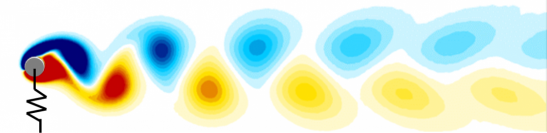
When the stiffness of the spring is very large, the cylinder can not move. For the low values of Reynolds number considered here, the wake flow is either steady (Re<47) or unsteady (Re >47). The unsteady wake is then characterized by the well-known Benard-Von Karman vortex-street, i.e an alternate shedding of vortices with opposite signs, which occurs spontaneously above the critical Reynolds number Rec=47. When the spring's stiffness and mass of the cylinder are such that the structural frequency is close to the vortex-shedding frequency (Strouhal number St ~ 0.1), the vortices induce large-amplitude vibrations of the cylinder and the shedding frequency then locks onto the structural frequency.
The so-called lock-in phenomenon is also observed for a spring-mounted cylinder at sub-critical Reynolds number (Re<47)., i.e for which the wake of the rigid cylinder is steady and does not exhibit any vortex street. Nevertheless, large-amplitude vibrations of the cylinder are obtained in a range of frequencies that depends on the fluid-to-solid density ratio. The figure below shows the maximal displacement of the cylinder obtained by numerical simulation of the unsteady flow exciting the spring-mounted cylinder, as a function of the structural frequency, for a fluid-to-solid denisity ratio equal to 50.

In the lock-in frequency region, the cylinder’s displacement continuously increases for smallest values of the structural frequencies while it decreases abruptly for largest values. Therr exist a range of structural frequency for which two solutions exist at the same frequency: a steady solution and an unsteady solution. The linear stability analysis developed below is useful to understand the destabilisation of the steady-state solution and to predict the critical structural frequencies. However, it does not explain the existence of multple steady-state solution. A weakly non-linear analysis of the psring-mounted cylinder flow can be performed around the critical values of the strucutral frequencies, to determine the supercritical or subcritial nature of the bifurcation, and to extimate the non-linear solutions close to these threshold values. To determine with accuracy the periodic solutions emerging from the bifurcation points, one propose to apply a frequency harmonic balance method.
Linear stability analysis
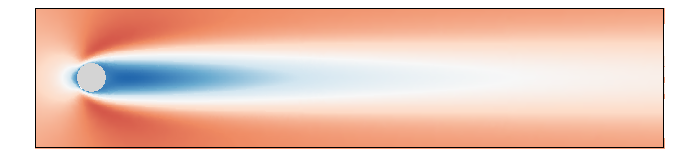
To understand why a displacement of the cylinder is observed for sub-critical values of the Reynolds number, a modal analysis of the spring-mounted cylinder flow is performed. We investigated the stability of the steady-state solution displayed in the figure below anbd corresponding to Re=40. The wake of the circular cylinder shown in grey is characeriozed by two recirculation regions symmetric with respect to the streawise axis.
The steady-state solution only depends on the Reynolds number, while its fluid-solid stability also depends on the solid-to-fluid density ratio  , the structural frequency < img style=" display: inline-block !important; height:25px;margin-bottom:-7px;margin-top:7px;width:76px;" alt="" src="https://w3.onera.fr/erc-aeroflex/sites/w3.onera.fr.erc-aeroflex/files/docs/olivier/viv-structuralfrequency.png">defined as the square root of the spring stiffness
  over the cylinder mass
  and the structural damping coefficient
  . In the following, the damping coefficient is fixed to
  , a rather small value. The fluid/solid stability analysis of the steady-state solution is first performed for three different values of the structural frequency. Physically speaking, the mass of the cylinder being constant, the stiffness of the spring is thus varied. The figure below shows the eigenvalue spectra.
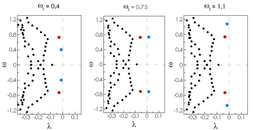
Two pairs of complex conjugate eigenvalue are highlighted in these figures with the blue and red dots. The red dots correspond to the eigenvalue of the leading fluid Wake Mode. They barely move in the complex plane when varying the structural frequency. For the Reynolds number Re=40 this eigenvalue lies in the stable half-plane. This result indicates that the steady solution is stable with respect to a purely fluid perturbation, in agreement with the hydrodynamic stability of this solution, obtained when considering only fluid perturbations. The frequency of this eigenvalue is  , close to the frequency of the vortex-shedding phenomenon in the wake of a fixed circular cylinder. The blue dots correspond to the eigenvalue of the Solid Mode. They move in the complex plane when carrying the structural frequency, with a frequency very close to the structural frequency . The structural damping being very small, the growth rate of this solid mode (blue dots) is expected to be slightly negative, but in a range of structural frequencies close to the vortex-shedding frequency ,this solid mode gets unstable, as for instance in the middle figure above.
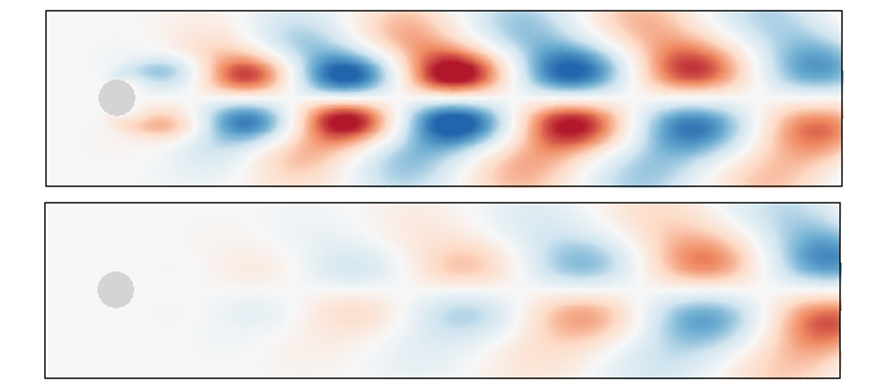
The spatial structures of the solid (top) and wake (bottom) mode are compared in the figure above, for the frequency  . They both exhibit an array of pair of patches symmetrically located with respect to the streamwise axis and of opposite sign. The sign of these patches also alternates in the streamwise direction, with a wavelength very similar in both cases, in agreement with the nearly identical frequency of the two modes. However, the magnitude of the streamwise velocity is larger for the solid Mode (top figure) than for the wake mode (bottom figure). When the frequency is varied, the spatial structure of the wake mode does not change, unlike the structure of the solid sode, as shown in the figures below.
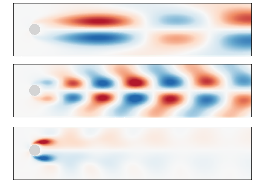
For the smaller structural frequency (top figure), the wavelength of the structure is larger. Note also that the first pair of structures immediately downstream the circular cylinder is of larger wavelength compred to those located further downstream in the wake. This reflects the existence of the recirculation regions in the steady solution that transports the perturbations. For the larger strucutral frequency (bottom figure), the fluid perturbation is large only in the very near proximity of the cylinder, and more specifically in the shear layer (of the steady solution) that develops immediately downstream the separation points on the cylinder’s wall. Further downstream in the wake, the array of positive and negative velocity’ patches is barely visible, indicating that the fluid perturbation is not spatially amplified at this frequency in the wake of the cylinder.
Turning now to the solid components of the eigenmode, we display in the figure below the absolute value of the vertical displacement of the cylinder, as a function of the structural frequency.
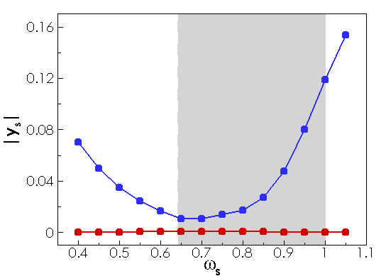
The vertical displacement of the solid mode (blue dots) is larger than the vertical displacement of the fluid wake mode (red dots) , which is weak for every structural frequency The region where the solid mode is unstable is displayed by the gray area in the figure. The displacement of the solid mode reaches a minimal value close to the lower critical frequency, and then increases with the structural frequency. We note that this increase of the vertical displacement component of the solid mode with the structural frequency is similar to the results obtained with the nonlinear temporal simulations and displayed in the second figure of this page. The comparison of these linear and nonlinear results should however be considered with caution.
The effect of the Reynolds number of the previous results is examined in the next figure, that displays the path of the solid and wake modes in the complex plane when the structural frequency is varied.
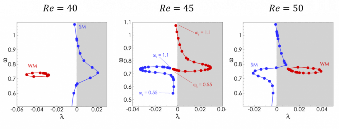
For the sub-critical value of the Reynolds number Re=40 (left figure), the wake mode is stable whatever the value of the structural frequency, while the solid mode gets unstable in a range of strucutral frequencies. For the super-critical value of the Reynolds number Re=50, the wake mode is unstable whatever the value of the structural frequency. The solid mode is first stabilized when increasing the structural frequency, and then gets unstable. In a range of frequency, there exist tow unstable eignemode. Finally, for the nearly critical value of the Reynolds number Re=45 displayed in the middle figure, it is not possible to make a clear distinction between the branch of solid mode and the branch of fluid wake mode. For instance, let us follow the path of the solid and fluid modes in the complex plane when increasing the structural frequency. For small strucutral frequency, the solid eigenvalue (blue) is slightly stable, and its frequency  is very close to the structural frequency, while the fluid eigenvalue (red dot) is also slightly stable but with a frequency close to the vortex-shedding frequency. Based on the values of the frequency, the blue and red eigenvalue correspond to the solid and fluid wake mode, respectively. Now, when the structural frequency is increased, the blue eigenvalue moves accordingly in the frequency direction, before being stabilized without a large change of frequency. For the largest value of structural frequency investigated here the blue eigenvalue has the frequency of the vortex shedding , and is almost at the position of the red eigenvalue obtained for the structural frequency This red eigenvalue gets first unstable when increasing the structural frequency from , without changing its own frequency When still increasing , the frequency of the red eigenvalue starts to increase, while its growth rate decreases. For the red eigenvalue lies in the stable half-plane and has the frequency close to the structural frequency. Clearly, the branches of blue and red eigenvalue cannot be characterized as the branch of solid and wake modes. It seems that they exchange their physical property when the structural frequency gets close to the “natural” vortex-shedding frequency.
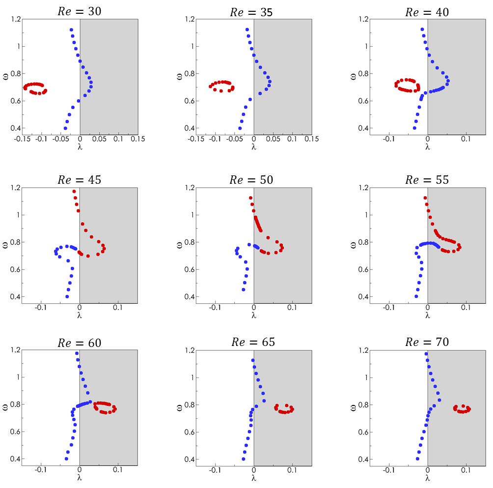
The evolution of the solid (blue) and wake (red) eigenvalues in the complex plane when varying the structural frequency is summarized in the figure below for various values of the Reynolds number.
Mean-state and extended mean-state analysis
In progress
Weakly non-linear analysis
In progress
Nonlinear analysis of limit cycles with the Harmonic Balance Method
The Harmonic Balance Method [1] is a numerical technique originally introduced to solve for time-periodic flows in forced system, for instance turbomachinary flows. This technique was extended to homogeneous time-periodic flows, i.e. stable and unstable limit cycles that are periodic solutions, arising from a Hopf bifurcation of the steady-state solutions. When considering large-scale problems, the Harmonic Balance Method is traditionnaly implemented using a Time Spectral approach. The purely frequency-based approach being limited to small-scale systems. Altohough we are dealing with a large-scale system, we have developed and implemented in the present sutdy a purely frequency-based approach.
References
[1] Hall K.C., Thomas J.P. and Clark W.S., Computation of unsteady nonlinear flows in cascades using a harmonic balance technique, AIAA Journal, Vol. 40, No 5, May 2002.
[2] Thomas J.P., Dowell E.H. and Hall K.C., Nonlinear inviscid aerodynamic effects on transonic divergence, flutter and limit-cycle oscillations, AIAA Journal, Vol. 40, No 4, April 2002.
[3] McMullen M.S., The application of non-linear frequency domain methods to the Euler and Navier-Stokes equations, PhD thesis, Stanford University, 2003.
[4] Thomas J.P., Dowell E.H. and Hall K.C., Modeling viscous transonic limit-cycle oscillation behavior using a harmonic balance approach, Journal of Aircraft, Vol. 41; No 6, November-December 2006.