Mathematical models are chosen to describe the fluid dynamics on one hand and the solid dynamics on the other hand. For the fluid, this choice depends on two non-dimensional numbers: the Mach number which determines whether the flow is compressible or incompressible, and the Reynolds number, which indicates whether the flow is laminar or turbulent. In the current state of the project, low Mach number flows are considered, so that the fluid motion is described as an incompressible viscous flow, and low and high Reynolds number flow cases are adressed. To describe the structural behaviour, two classes of models are considered: rigid solids mounted on springs, as classicaly done in aeroelasticity or civil engineering studies, and deformable structures made of hyperelastic materials.
Fluid modeling
We consider viscous Newtonian fluids and describe their motion in an Eulerian framework with the Navier-Stokes equations. Models of increasing complexity are used, depending on the physical parameters.
- Incompressible laminar flows
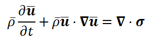
When the Reynolds number Re and Mach number Ma are small, the flow is incompressible and described by the laminar Navier-Stokes equations. The conservative form of the momentum equation is
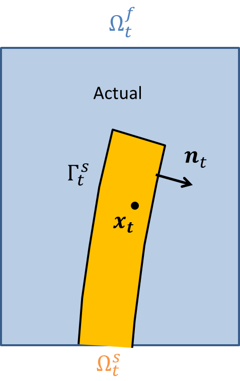
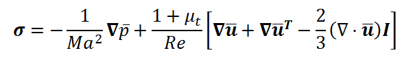
where uE (xt,t) is the Eulerian velocity field, i.e. the velocity of the fluid at the spatial position xt of the fluid domain. In fluid/structure interaction problems, the fluid domain moves as a result of the solid motion and thus the spatial coordinate xt is time dependent, as indicated by the subscript. This time dependence of the spatial domain is also indicated in the spatial derivative operator with the subscript t. For a Newtonian incompressible viscous fluid, the Cauchy stress tensor is defined as
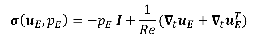
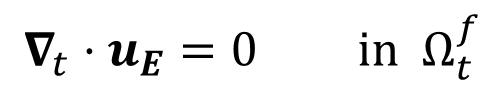
Mathematically speaking, the pressure field pE is a Lagrangian multiplier associated to the divergence-free constraint
- Incompressible turbulent flows
When the Mach number Ma is small but the Reynolds number Re is large, the flow is incompressible and turbulent. The flow velocity is then decomposed as the sum of a mean component and a fluctuating component, i.e.

The mean component is then governed by the incompressible Reynolds Averaged Navier Stokes (RANS) equations
which differs from the Navier-SDtokes equations by an additional stress term. The so-called turbulence Reynolds stresses depend quadratically on the fluctuating velocity field, which is unknown. To close the problem, the turbulence Reynolds stresses are modelled as a function of the mean velocty and pressure component, solely. Using he Boussinesq approximation, which introduces an eddy viscosity field, the unsteady Reynolds Averaged Navier-Stokes (RANS) equations write
where  is the turbulence eddy viscosity, determined with a turbulence model. The Spalart-Allmaras turbulence model is a one-equation model that solves a transport equation for a surrogate viscosity.
- Compressible turbulent flows
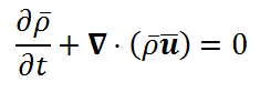
When the Reynolds number Re and Mach number Ma are large, the flow is compressible and turbulent. It is then described by the compressible unsteady Reynolds Averaged Navier-Stokes (RANS) equations
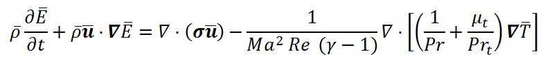
\mut represents the turbulent viscosity to be computed through some RANS turbulence model (e.g. Spalart-Allmaras).
Solid modeling
We introduce here the notation for modelling rigid structures mounted on spring and the structural model used for the nonlinear elastic material.
- Spring-mounted rigid cylinder
Add a scketch of the srping-mounted clyinder (similar to what Johann did)
The evolution equation of the vertical displacement of the mass center is a damped harmonic oscillator forced by the y-component of the aerodynamical force
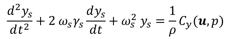
where  is the vertical displacement of the cylinder's mass center,
  is the structural frequency, defined as the square root of the spring's stiffness over the cylinder's mass,
  is the (structural) damping coefficient and
  is the solid-to-fluid denisty ratio.
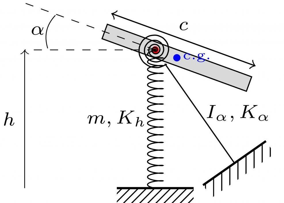
- Translational and torsional spring-mounted rigid plates
A very simple modelisation of a moving solid consists in considering a rotating and translating rigd body. For example, when a rigid solid is allowed to translate in the vertical direction and rotate around some elastic axis, simple equations of motion based on harmonic oscillators are obtained :
 is the lift force (positive upwards)
 is the moment of fluid forces evaluated at the elastic center (chosen positive nose-down here)
 is the static unbalance. Note that if the center of gravity is not aligned with the elastic axis, the heaving and pitching degrees of freedom are inertially coupled through the static unbalance term.
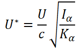
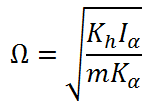
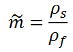
The following set of non-dimensional numbers can be used to describe this system :
Image
| Image
| Image
| Image
|
Ref : E. Dowell, H. Curtiss, R. Scanlan, A modern Course in Aeroelasticity, Fifth Revised and Enlarged Edition, Springer, 2015
- Linear and nonlinear elastic solids
The evolution of an elastic structure is defined by the motion of its material points. The position  of any material point in the actual configuration is defined with respect to its position in a reference configuration. In solid mechanics, a natural choice for this reference configuration is the spatial domain occupied by the solid when no external stresses are applied. We will denote
  the spatial position configuration in this reference configuration. Other choices for the reference configuration could be made, especially when investigating the stability analysis.
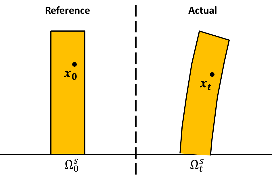
The material displacement is a Lagrangian field defined as the difference between the actual position and the reference position, i.e.
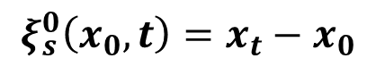
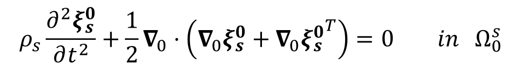
and the solid dynamics is described by the evolution equation of the displacement field
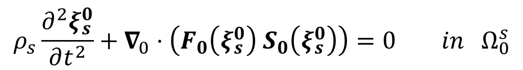
where  is the solid density,
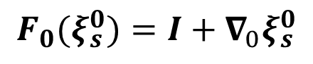
  is the deformation gradient of the solid defined as
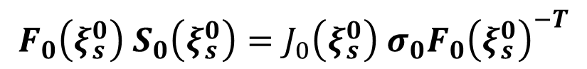
and  is the second Piola-Kirchhoff stress tensor. The second Piola-Kirchhoff stress is classically used in solid mechanics since it is a measure of the force acting on an element of area in the reference configuration, as opposed to the Cauchy stress tensor, classically used in fluid mechanics, since it is a measure of the force acting on an element of area in the actual configuration. The Cauchy and second Piola-Kirchhoff stress tensors are related through the formula
where  , the determinant of the deformation gradient
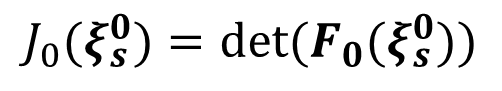
measures the volumic change of the solid and is equal to unity in case of an incompressible solid.
In the AEROFLEX project, we mainly consider hyperelastic materials modelled with the Saint Venant-Kirchhoff law, which relates the second Piola-Kirchhoff stress tensor to the displacement field
via the Green-Lagrangian strain tensor defined as
This is a model valid for small deformations and large displacements of an elastic solid. In case of small displacements, the quadratic (nonlinear) term in the Green-Lagrangian stress tensor is negligible and the equation governing the solid dynamics reduces to the classical linear elasticity equation
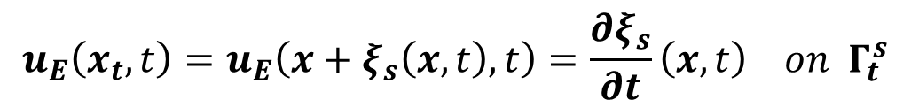
Fluid/Elastic solid coupling
The fluid and solid dynamics are naturally described by variables of different nature. The fluid velocity is an Eulerian variable that describes the velocity of the fluid at a fixed spatial position in space, while the solid displacement is a Lagrangian variable that describes the displacement of a material point in a fixed reference configuration. The complexity in the modelling of fluid/structure interaction problem arises from the coupling between the Eulerian fluid and Lagrangian solid description.

To cope with the coupling of the Eulerian and Lagrangian description, various strategies have emerged in the literature dealing with the numerical resolution of the unsteady nonlinear fluid/solid equation. They can be classified into two class of methods: the conforming methods and the non-conforming methods. In the present project, the coupling of the nonlinear fluid/solid equations is described either within an Arbitrary Lagrangian Eulerian (ALE) framework (conforming method) or with a Fictitious Domain approach (non-conforming method).
References:
G. Hou, J. Wang and A. Layton, Numerical Methods for Fluid Structure interaction – A review, Communication in Computational Physics, Vol 12, No 2, pp. 337-377