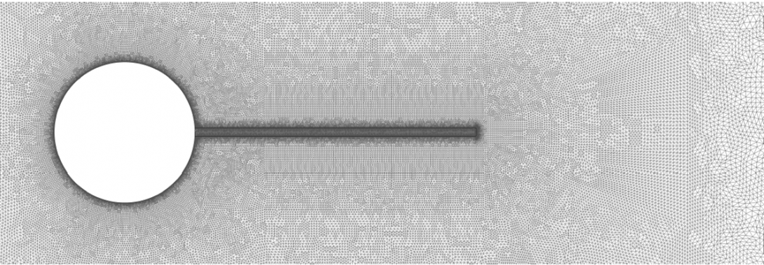
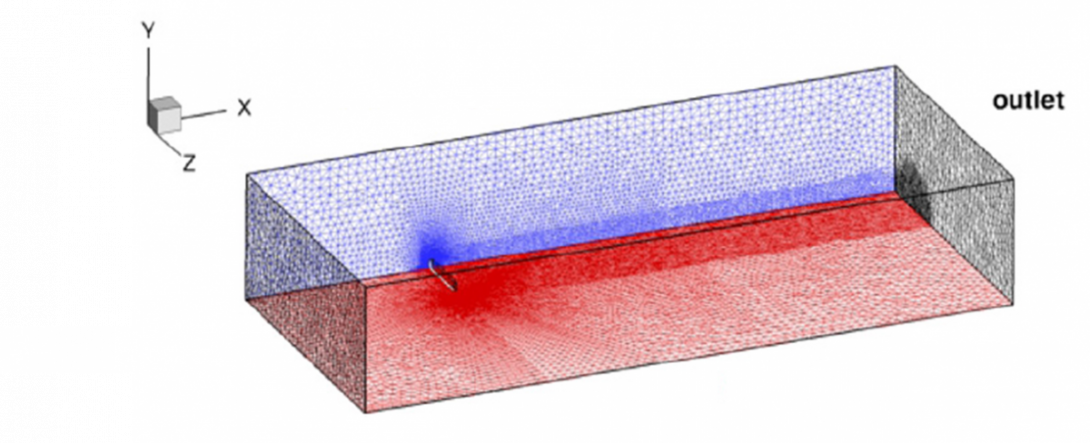
The partial differential equations governing the fluid and solid dynamics are discretized using the finite-element method. The meshes are made of triangles for two-dimensional configurations and of tetrahedra for three-dimensional configurations.
The finite-element method is based on a derivation of the weak formulation of the governing equations. This weak formulation is then discretized using the free software FreeFem++ that enables a spatial discretization of partial differential equations using the Finite Element method. The incompressible Navier-Stokes equations are discretized using Taylor-Hood elements: the fluid velocity is discretized with continuous quadratic functions (P2) while the pressure is discretized with continuous linear functions (P1). To discretize the elasticity equations as a first-order problem in time, the solid velocity field is introduced as an additional variable. The solid displacement and velocity are then discretized with continuous quadratic functions, so that the fluid and solid velocities are dfiscretized by continuous function of similar order at the interface. In the ALE formulation, the extension displacement field, introduced to handle the deformation of the fluid mesh, is also discretized with continuous quadraticelement (P2), so that the solid displacement and extension displacement are discretized at the interface with elements of same order. Two Lagrange multiplier fields are defined on the fluid-solid interface: one to enforce the continuity of the fluid and solid velocities at the fluid-solid interface, and one to enforce the continuity of the solid and extension displacement. These two Lagrange multiplier fields are discretized with continuous linear function (P1) for numerical stability reason.
ALE formulation - Lagrangian decomposition
The spatial discretization of the eigenvalue problem obtained when considering the decomposition of the Lagrangian fluid velocity field is

where the fluid, extension and solid unknows are
and  ,
, are the two Lagrange multipliers discussed above. The fluid-structure-extension matrix is composed of the on-diagonal matrices: Af the Jacobian matrix of the fluid equations, As the discretize operator of the linear elastic equation and Ae the discretized extension operator. The off-diagonal matrices couple the fluid, extension and solid equations. In the first line (fluid equation) the matrix Cfs is a mass matrix defined on the fluid-solid boundary while the matrix Cfe represent the shape derivative of the fluid equation. In the extensnion equation, Ces is also a mass matrix defined on the fluid-solid boundary. Interestingly, the matrix on the right hand-side is not symmetric due to the presence of the matrix Bfe. The fluid mesh velocity would be defined as an additional variable, the matrix on the right hand-side would be symmetric.
ALE formulation - Eulerian decomposition
The decomposition of the Eulerian fluid velocity filed yields to the following discretized eigenvalue problem

where the extension displacement variable has been eliminated. Two new matrices appear in this formulation: the matrix T discretize the transpiration velocity operator on the lfuid-solid boundary while the matrix K0 discretizes the added-stiffness terms.