Model description
The following equations describe the longitudinal motion of a rigid aircraft [1] in body axis ($x$ forwards and $z$ downwards): $$\left\{\begin{array}{lcl}mV\dot{\alpha} & = & mVq-\frac{\rho SV^2}{2}C_L-F_{eng}\sin\alpha+mg\cos\gamma \\ I_{yy}\dot{q} & = & \frac{\rho SV^2}{2}\Big[ LC_M+\delta x\left(C_L\cos\alpha+C_D\sin\alpha\right)\Big] +\delta zF_{eng}\end{array}\right.$$ The flight parameters are the angle of attack $\alpha$, the pitch rate $q$, the airspeed $V$, and the flight path angle $\gamma$. The constants are denoted by $g$ (gravity), $\rho$ (air density), $m$ (aircraft mass), $S$ (reference surface), $I_{yy}$ (lateral $y$-axis inertia), and $L$ (mean aerodynamic chord). $F_{eng}$ is the thrust, whereas $\delta x=x_{ref}-x_{cg}$ and $\delta z=z_{eng}-z_{ref}$ represent the distances between the aerodynamic reference point and the centre of gravity $x$-location or the engine $z$-location.
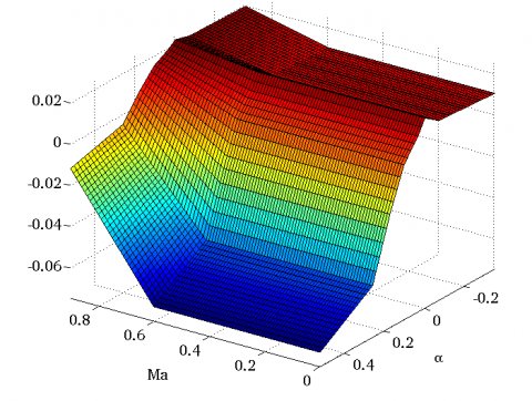
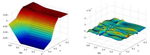
$C_L,C_D$ and $C_M$ represent the aerodynamic coefficients relative to the lift, drag and pitching moments. They are usually obtained as nonlinear look-up tables during wind tunnel tests. In order to translate the above equations in fractional form, these tabulated data have to be replaced by polynomial or rational expressions, which can be achieved using any of the approximation methods implemented in the APRICOT Library of the SMAC Toolbox. This is illustrated below for the drag coefficient $C_D$ of a generic fighter aircraft model [2]. The reference data depend on both the Mach number $Ma$ and the angle of attack $\alpha$ (in radians). They are given on a fine 50x90 grid and are represented in Figure 1.
The goal is to achieve the simplest possible approximation, while ensuring that the Root Mean Square Error (RMSE) between approximant and reference data remains close to a given value $\epsilon$ on the grid.
Polynomial approximation
Polynomial approximation is considered first. All results are gathered in Tables 1 and 2, which correspond to $\epsilon\approx 2\;10^{-3}$ and $\epsilon\approx 9\;10^{-4}$ respectively. The third and the forth columns specify the degree of the polynomial function used for approximation, as well as the total number of monomials when both the numerator and the denominator are expanded. The RMSE and the maximum local error $\epsilon_{max}=\max_{k\in [1,N]} |y_k-f(x_k)|$ are then given in the fifth and the sixth columns respectively. The complexity of the resulting LFR is finally measured via the size of its $\Delta$ matrix in the last column.
| Approximation method | Routine | Degree | Monomials | RMSE | Max error | LFR size |
| linear least-squares [3] | lsapprox | $6$ | $28$ | $1.94\;10^{-3}$ | $8.94\;10^{-3}$ | $12$ |
| orthogonal least-squares [4,5] | olsapprox | $6$ | $21$ | $2.17\;10^{-3}$ | $1.01\;10^{-2}$ | $9$ |
Table 1. Comparison of the polynomial approximation techniques for $\epsilon\approx 2\;10^{-3}$
| Approximation method | Routine | Degree | Monomials | RMSE | Max error | LFR size |
| linear least-squares [3] | lsapprox | $12$ | $91$ | $9.20\;10^{-4}$ | $4.84\;10^{-3}$ | $24$ |
| orthogonal least-squares [4,5] | olsapprox | $12$ | $54$ | $9.65\;10^{-4}$ | $5.54\;10^{-3}$ | $20$ |
Table 2. Comparison of the polynomial approximation techniques for $\epsilon\approx 9\;10^{-4}$
The orthogonal least-squares based algorithm allows to generate sparse expressions. Both the number of monomials and the size of the resulting LFR can be reduced with no significant loss of accuracy.
Rational approximation
The most classical rational approximation techniques are now compared for the same values of ε. All results are gathered in Tables 3 and 4. Note that both methods generate full expressions in the sense that all admissible monomials are nonzero.
| Approximation method | Routine | Degree | Monomials | RMSE | Max error | LFR size |
| nonlinear least-squares [6] | cftool | $3$ | $20$ | $1.90\;10^{-3}$ | $5.71\;10^{-3}$ | $8$ |
| quadratic programming [7] | qpapprox | $3$ | $20$ | $1.77\;10^{-3}$ | $5.62\;10^{-3}$ | $8$ |
| quadratic programming [7] | qpapprox | $5\ (2$-$3)$ | $24$ | $1.67\;10^{-3}$ | $4.95\;10^{-3}$ | $7$ |
Table 3. Comparison of the most classical rational approximation techniques for $\epsilon\approx 2\;10^{-3}$
| Approximation method | Routine | Degree | Monomials | RMSE | Max error | LFR size |
| nonlinear least-squares [6] | cftool | $6$ | $56$ | $9.15\;10^{-4}$ | $3.51\;10^{-3}$ | $17$ |
| quadratic programming [7] | qpapprox | $6$ | $56$ | $9.05\;10^{-4}$ | $3.51\;10^{-3}$ | $17$ |
| quadratic programming [7] | qpapprox | $8\ (3$-$6)$ | $54$ | $7.22\;10^{-4}$ | $2.93\;10^{-3}$ | $12$ |
Table 4. Comparison of the most classical rational approximation techniques for $\epsilon\approx 9\;10^{-4}$
Both algorithms provide very similar results. Moreover, it appears that rational approximation is more efficient than polynomial approximation, since both the number of monomials and the size of the resulting LFR are lower. Finally, note that quite good results can sometimes be obtained by increasing the degree of the approximating function but limiting the maximum exponent of each variable. For example, in the last line of Table 3 (resp. Table 4), both the errors and the size of the LFR are quite low with a rational function of degree 5 (resp. 8) for which the maximum exponents of $Ma$ and $\alpha$ are 2 and 3 (resp. 3 and 6).
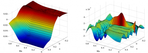
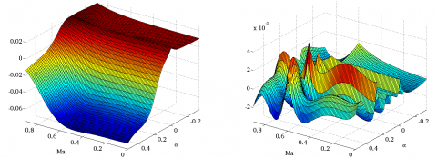
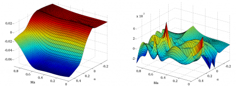
The most recent techniques for rational approximation are finally compared with the aforementioned quadratic approach, which gives the best results so far. All results are gathered in Table 5, and some are also displayed in Figures 2 and 3. For the surrogate modeling based algorithm, the number of monomials is given both for the factorized expression obtained with the routine koala (without brackets) and for the associated expanded form (between brackets).
| Approximation method | Routine | Degree | Monomials | RMSE | Max error | LFR size |
| quadratic programming [7] | qpapprox | $4$ | $30$ | $1.60\;10^{-3}$ | $4.72\;10^{-3}$ | $11$ |
| $6$ | $56$ | $9.05\;10^{-4}$ | $3.51\;10^{-3}$ | $17$ | ||
| $8$ | $90$ | $6.06\;10^{-4}$ | $2.69\;10^{-3}$ | $23$ | ||
| genetic programming [8] | tracker | $6$ | $30$ | $9.74\;10^{-4}$ | $4.60\;10^{-3}$ | $14$ |
| $8$ | $25$ | $8.73\;10^{-4}$ | $4.71\;10^{-3}$ | $15$ | ||
| $14$ | $43$ | $6.53\;10^{-4}$ | $3.05\;10^{-3}$ | $28$ | ||
| surrogate modeling [9] | koala | $6$ | $18\ (46)$ | $1.28\;10^{-3}$ | $6.23\;10^{-3}$ | $12$ |
| $8$ | $24\ (77)$ | $7.92\;10^{-4}$ | $5.12\;10^{-3}$ | $16$ | ||
| $14$ | $42\ (218)$ | $3.55\;10^{-4}$ | $1.96\;10^{-3}$ | $28$ | ||
| $26$ | $78\ (716)$ | $1.58\;10^{-4}$ | $1.03\;10^{-3}$ | $52$ |
Table 5. Comparison of the most avanced rational approximation techniques
Genetic programming has a great advantage, since it creates rational approximants with sparse structures. Only a few monomials are actually nonzero, which results in low-order LFR. Moreover, good numerical properties are observed, and significantly higher degrees can be considered than with quadratic programming.
For a given degree, surrogate modeling and quadratic programming give quite similar results regarding the number of monomials. Indeed, both methods generate rational functions for which the numerator and the denominator are composed of almost all admissible monomials when written in expanded form. But surrogate modeling offers two major pros. First, the size of the resulting LFR is smaller, since the symbolic expression does not appear as a single expanded rational function, but is already factorized as a sum of elementary components. Besides, surrogate modeling is numerically much more efficient and allows to compute higher degree approximations very quickly and easily. This is not possible with quadratic programming, since numerical troubles appear for degrees larger than 8, thus leading to poor results.
Genetic programming and surrogate modeling thus appear to be the most efficient methods on this example. Moreover, these two methods prove quite complementary. Surrogate modeling provides very accurate approximations, which do not have a sparse structure but can be directly factorized in a compact form resulting in low order LFR. On the other hand, genetic programming directly selects the most relevant monomials to generate very sparse symbolic expressions. It also appears that genetic programming is more accurate for low degree approximations, while surrogate modeling gives better results for degrees larger than 8. Indeed, at lower degrees, the number of radial units used by the latter method (half the required degree) is not sufficient to represent accurately enough the shape of the reference data. Hence, a minimum number of radial basis functions is required to get the most out of this method. Finally, it is worth noting that the computational cost is strongly in favor of the surrogate modeling based algorithm. As the degree of the rational function increases, the Darwinian mechanisms of evolution involved by genetic programming require more generations to produce very accurate solutions, and the CPU time is seriously impaired.
Remark: It is worth emphasizing that the non singularity of the rational functions is guaranteed in all cases.
Figure 2: Approximants of degree 8 and local approximation errors (top = quadratic programming, middle = genetic programming and bottom = surrogate modeling)
Figure 3: Approximant of degree 26 and local approximation error (surrogate modeling)
References
| [1] | J-L. Boiffier, The dynamics of flight: the equations, John Wiley & sons, Chichester, 1998. |
| [2] | C. Döll, C. Bérard, A. Knauf and J-M. Biannic, "LFT modelling of the 2-DOF longitudinal nonlinear aircraft behaviour", in Proceedings of the 9th IEEE Symposium on Computer-Aided Control System Design, San Antonio, Texas, September 2008, pp. 864-869. |
| [3] | J-F. Magni, User manual of the Linear Fractional Representation Toolbox (version 2.0), available at http://www.onera.fr/fr/staff/jean-marc-biannic?page=3, 2006. |
| [4] | C. Poussot-Vassal and C. Roos, "Generation of a reduced-order LPV/LFT model from a set of large-scale MIMO LTI flexible aircraft models", Control Engineering Practice, vol. 20, no. 9, pp.919-930, 2012. |
| [5] | C. Roos, "Generation of flexible aircraft LFT models for robustness analysis", in Proceedings of the 6th IFAC Symposium on Robust Control Design, Haifa, Israel, June 2009. |
| [6] | The Mathworks, Curve fitting toolbox user's guide, 2010. |
| [7] | O.S. Celis, A. Cuyt and B. Verdonk, "Rational approximation of vertical segments", Numerical Algorithms, vol. 45, no. 1-4, pp. 375-388, 2007. |
| [8] | G. Hardier, C. Roos and C. Seren, "Creating sparse rational approximations for linear fractional representations using genetic programming", in Proceedings of the 3rd IFAC International Conference on Intelligent Control and Automation Science, Chengdu, China, September 2013, pp. 232-237. |
| [9] | G. Hardier, C. Roos and C. Seren, "Creating sparse rational approximations for linear fractional representations using surrogate modeling", in Proceedings of the 3rd IFAC International Conference on Intelligent Control and Automation Science, Chengdu, China, September 2013, pp. 238-243. |

