A new Matlab class to model uncertain and nonlinear systems | SMAC

Please report any problems to Clément Roos (croos@onera.fr) or Jean-Marc Biannic (biannic@onera.fr). We will try to fix them as quickly as possible!

Overview

The GSS library (Generalized State Space) of the SMAC toolbox implements a new Matlab class, which allows to model uncertain and nonlinear systems as Linear Fractional Representations. It replaces and extends the LFR toolbox, with a more intuitive way to describe LFR and a more user-friendly interface, including a Simulink library. Several tools are proposed to manipulate GSS objects (addition, multiplication, inversion, concatenation, feedback...), obtain GSS objects from symbolic models, convert GSS/LFR/USS objects, manipulate the uncertainties and the nonlinearities (normalization, reordering, random sampling), and perform order reduction or approximation. A large class of continuous- and discrete-time systems can be handled, with real or complex uncertain or varying parameters, polytopic-type uncertain or varying elements, linear time-invariant uncertainties, sector nonlinearities, saturations, deadzones, or more general nonlinear operators. Full compatibility is also ensured with other modeling, analysis and control libraries of the SMAC toolbox (APRICOT, SMART, IQC, SAW...).

Matlab GSS object description

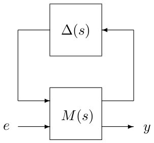
Linear Fractional Representations are a straightforward extension of state-space models with uncertain elements, parametric variations, and isolated nonlinearities. They consist of a continuous- or discrete-time LTI model $M(s)$ or $M(z)$ in feedback loop with a block diagonal operator $\Delta=\textrm{diag}(\Delta_1,\dots,\Delta_N)$ which collects uncertain, varying and nonlinear elements:

perf — Figure 1: Linear Fractional Representation

Each $\Delta_i$ block can be a real or complex uncertain or varying parameter (PAR), a polytopic-type uncertain or varying element (POL), a linear time-invariant system (LTI), a sector nonlinearity (SEC), a saturation (SAT), a deadzone (DZN) or any other nonlinear operator (NLB). The GSS library of the SMAC toolbox implements a new Matlab class. It allows to describe a Linear Fractional Representation as a GSS object, which is a structured variable with two fields:

M: SS/TF/ZPK object representing the LTI model $M(s)$ or $M(z)$.
D: $1\times N$ structured array describing each $\Delta_i$ block with fields

`Name`	Name of the block	String with no trailing underscore
`Type`	Type of the block (see above)	String `'PAR'`, `'POL'`, `'LTI'`, `'SEC'`, `'SAT'`, `'DZN'` or `'NLB'`
`Size`	Size of the block	Number of rows and columns $[n_{row}\ n_{col}]$
`NomValue`	Nominal value	real `PAR`: real number $p_{nom}$ complex `PAR`: real or complex number $p_{nom}$ `POL`: 0 or $n_{row}\hspace{-0.5mm}\times\hspace{-0.5mm} n_{col}$ matrix `LTI`: 0 or $n_{row}\times n_{col}$ matrix or $n_{row}\times n_{col}$ SS/TF/ZPK object `SEC`: nominal slope $k_{nom}$ `SAT`, `DZN` and `NLB`: no predefined format
`Bounds`	Bounds information	real `PAR`: minimum and maximum values $[p_{min}\ p_{max}]$ complex `PAR`: 1x3 vector $[c_{re}\ c_{im}\ r]$ defining a circle in the complex plane of center $c_{re}+c_{im}i$ and of radius $r>0$ `POL`: $n_{row}\hspace{-0.5mm}\times\hspace{-0.5mm} n_{col}\hspace{-0.5mm}\times\hspace{-0.5mm} n_{ver}$ matrix corresponding to $n_{ver}$ vertices of a polytope `LTI`: scalar $b>0$ such that $\\|\Delta_i\\|_\infty < b$ or SISO causal SS/TF/ZPK object $B$ defining a frequency dependent bound such that $\sigma_{max} (\Delta_i(\omega)) < \|B(\omega)\|$ for all $\omega$ `SEC`: minimum and maximum slopes $[k_{min}\ k_{max}]$ `SAT`, `DZN` and `NLB`: no predefined format
`RateBounds`	Bounds on the rate of variation	`PAR`: minimum and maximum rates $[r_{min}\ r_{max}]$ `POL`, `LTI`, `SEC`, `SAT`, `DZN` and `NLB`: no predefined format
`Measured`	Indicates whether a block can be measured or not	String `'yes'` or `'no'`
`Normalization`	Stores bounds information in case of normalization	`PAR` and `LTI`: same format as the field `Bounds` (see the routine `dbnorm` for more information) `POL`, `SEC`, `SAT`, `DZN` and `NLB`: no predefined format
`Misc`	Can be used to store any additional data	No predefined format

The fields Name, Type and Size must be specified for each block, whereas the other fields can be left empty.

Matlab GSS object generation

There are several ways to create a GSS object.

Conversion of an existing object
sys=gss(sys1)
The input argument sys1 can be a GSS object, a LFR object obtained with the LFR toolbox, a USS object obtained with the Robust Control toolbox, a SS/TF/ZPK object or a standard matrix. Note that the call sys=gss can be used to create an empty GSS object.
Creation from variables M and D
sys=gss(M,D)
M is a SS/TF/ZPK object or a numeric array. D is a $1\times N$ structured array with fields Name, Type, Size, NomValue, Bounds, RateBounds, Measured, Normalization and Misc. Name must be defined for each $\Delta_i$ block, whereas the other fields can be empty or omitted. Note that Type and Size are set to 'PAR' and [1 1] respectively if empty or omitted.
Creation of elementary GSS objects with a single block
1. Creation by properties and values sys=gss('Property1',Value1,'Property2',Value2,...)
  The allowed properties are Name, Type, Size, NomValue, Bounds, RateBounds, Measured, Normalization and Misc. Only Name has to be defined. If undefined, Type and Size are set to 'PAR' and [1 1] respectively, whereas the other properties are left empty. Example: a=gss('Name','a','Type','PAR','Size',[1 1],'Bounds',[2 4])
2. Creation by values only sys=gss(Name,Type,Size,NomValue,Bounds,RateBounds,Measured,Normalization,Misc) The values must be given in the right order, but some of them can be empty and the last ones can be ignored. Only Name has to be defined. If undefined, Type and Size are set to 'PAR' and [1 1] respectively, whereas the other properties are left empty. Example: a=gss('a','PAR',[1 1],[],[2 4])
3. Use of a simplified call in the parametric case sys=gss(Name,NomValue,Bounds,RateBounds) The values must be given in the right order, but some of them can be empty and the last ones can be ignored. Only Name has to be defined. Type, Size, Measured, Normalization and Misc are set to 'PAR', [1 1], 'no', [] and [] respectively. RateBounds is set to [0 0] if undefined. NomValue and Bounds are set to 0 and [-1 1] if none are defined, whereas NomValue is set to mean(Bounds) if only Bounds is defined and Bounds is set to [NomValue-1 NomValue+1] if only NomValue is defined. Example: a=gss('a',[],[2 4])
Starting from R2014b, the output argument can be omitted when an elementary GSS object is created. In other words, gss('a',[],[2 4]) is a shortcut for a=gss('a',[],[2 4]).
Use of the reserved names Int and Delay Int and Delay can be used to create elementary GSS objects such that $M(s)=1/s$ and $M(z)=1/z$ respectively, and $\Delta$ is empty. Example: Int=gss('Int')
Interconnection of GSS objects The overloaded routines plus, minus, uminus, mtimes, inv, mrdivide, mldivide, mpower, horzcat, vertcat, append, ctranspose, transpose, ss, tf and feedback can be applied to GSS objects. Type 'help gss/rname' to get detailed information about the routine rname.
Application of the structured tree decomposition algorithm to a symbolic polynomial expression to obtain a low order GSS object. Type 'help sym2gss' to get detailed information.
Sparse polynomial or rational approximation to obtain a low-order GSS object from tabulated data. Type 'help data2gss' to get detailed information. See also the APRICOT library.

Warning: A systematic order reduction is performed by default with the routine mingss each time a GSS object is created or an elementary operation is applied to an existing GSS object (addition, multiplication, division, concatenation...). This setting can be changed using the routine setred.

Warning: No systematic normalization is performed by default, but PAR and LTI blocks are normalized in case of inversion or inconsistency problem with the routine dbnorm. This setting can be changed using the routine setnorm.

Warning: In case of an unexpected error, use the routine checkgss to check whether the considered GSS objects are consistent.