
This simple example shows how the GSS library with the GSSLIB Simulink interface can be used to design a controller for a nonlinear uncertain system and to perform a basic robustness analysis.
Problem statement
The considered open-loop plant is the series interconnection of:
- a 1st order actuator with uncertain time constant and position limits,
- a 2nd order system with uncertain frequency and damping.
\begin{equation} \left\{\begin{array}{ccl}\dot{x_1}&=&-\color{darkgreen}{\tau} x+u\\[4pt]v&=&\color{red}{\textrm{sat}_{[-2,3]}(}x_1\color{red}{)}\\[4pt]\color{darkgreen}{\tau}&\color{darkgreen}{\in}&\color{darkgreen}{[\begin{array}{cc}0.08&0.12\end{array}]}\end{array}\right. \hspace{3cm} \left\{\begin{array}{ccl}\ddot{x_2}&=&-2\color{orange}{\xi\omega}\dot{x_2}-\color{orange}{\omega^2}x_2+\color{orange}{\omega^2}v\\[4pt]y&=&\left[\begin{array}{cc}x_2&\dot{x_2}\end{array}\right]^T\\[4pt]\color{orange}{\omega}&\color{orange}{\in}&\color{orange}{[\begin{array}{cc}1&3\end{array}]}\\[4pt]\color{orange}{\xi}&\color{orange}{\in}&\color{orange}{[\begin{array}{cc}0.1&0.5\end{array}]}\end{array}\right. \end{equation} The objective is to design a PID controller such that the uncertain closed-loop plant behaves like a second-order system with frequency > 1 rad/s and damping > 0.7.
The objective is to design a PID controller such that the uncertain closed-loop plant behaves like a second-order system with frequency > 1 rad/s and damping > 0.7.
Creation of the open-loop GSS object
The actuator with uncertain time constant and position limits is modeled first:
>> sat=gss('position','SAT',[1 1],1,[-2 3]);>> tau=gss('tau',0.1,[0.08 0.12]);>> actuator=sat*tf(1,[tau 1]);>> size(actuator)
Warning: Normalization has been performed to avoid inversion problems.
Continuous-time GSS object actuator with 1 output, 1 input and 1 state.
2 blocks in Delta: global size = 2x2.Name Type Size Measured NomValue Boundsposition SAT 1x1 ? 1 limits = [-2 3]tau PAR (real) 1x1 no 0 min/max = [-1 1]
The second-order system with uncertain frequency and damping is defined next. First solution: the state-space matrices are defined as gss objects. >> xi=gss('damping',0.3,[0.1 0.5]);>> omega=gss('frequency',2,[1 3]);>> A=[0 1;-omega^2 -2*xi*omega];>> B=[0;omega^2];>> C=[1 0;0 1];>> D=[0;0];
They are turned into a dynamic model.
>> setred('no')>> sys1=ss(A,B,C,D);>> size(sys1)
Continuous-time GSS object sys1 with 2 outputs, 1 input and 2 states.
2 blocks in Delta: global size = 6x6.Name Type Size Measured NomValue Boundsdamping PAR (real) 1x1 no 0.3 min/max = [0.1 0.5]frequency PAR (real) 5x5 no 2 min/max = [1 3]
$\Rightarrow$ frequency is repeated 5 times if no order reduction is performed.
>> setred('default')>> sys1=ss(A,B,C,D);>> size(sys1)
Continuous-time GSS object sys1 with 2 outputs, 1 input and 2 states.
2 blocks in Delta: global size = 4x4.
Name Type Size Measured NomValue Bounds
damping PAR (real) 1x1 no 0.3 min/max = [0.1 0.5]
frequency PAR (real) 3x3 no 2 min/max = [1 3]
$\Rightarrow$ frequency is repeated 3 times if order reduction is performed.
Second solution: The state-space matrices are defined as symbolic objects.
>> syms frequency damping>> A=[0 1;-frequency^2 -2*damping*frequency];>> B=[0;frequency^2];>> C=[1 0;0 1];>> D=[0;0];
They are turned into a dynamic model.
>> abcd=sym2gss([A B;C D]);>> sys2=abcd2gss(abcd,2);>> set(sys2,'damping','NomValue',0.3,'Bounds',[0.1 0.5]);>> set(sys2,'frequency','NomValue',2,'Bounds',[1 3]);>> size(sys2)
Continuous-time GSS object sys2 with 2 outputs, 1 input and 2 states.
2 blocks in Delta: global size = 3x3.Name Type Size Measured NomValue Boundsdamping PAR (real) 1x1 no 0.3 min/max = [0.1 0.5]frequency PAR (real) 2x2 no 2 min/max = [1 3]
$\Rightarrow$ frequency is repeated twice, which corresponds to the minimal realization.
It can be checked that the two gss objects are equivalent.
>> distgss(sys1,sys2)
$\Rightarrow$ the returned value is zero!
The gss object sys2 is simpler and is thus considered in the sequel.
>> sys=sys2;
The linearized open-loop plant is analyzed. The saturation is ignored and 200 random samples are computed.
>> sys_lin=eval(sys,'position','nominal');>> [sys0,samples]=dbsample(sys_lin,200);>> figure,hold on,grid on>> for k=1:length(sys0)>> ev=eig(sys0{k});>> plot(real(ev),imag(ev),'b.')>> end>> xlim([-1.8 0.3]);>> ylim([-4 4]);>> plot(-0.1*[1 3],sqrt(1-0.1^2)*[1 3],'r-')>> plot(-0.1*[1 3],-sqrt(1-0.1^2)*[1 3],'r-')>> plot(-0.5*[1 3],sqrt(1-0.5^2)*[1 3],'r-')>> plot(-0.5*[1 3],-sqrt(1-0.5^2)*[1 3],'r-')>> theta=1.671:0.001:2.095;>> plot(cos(theta),sin(theta),'g-')>> plot(3*cos(theta),3*sin(theta),'g-')>> plot(cos(-theta),sin(-theta),'g-')>> plot(3*cos(-theta),3*sin(-theta),'g-')>> xlabel('real part')>> ylabel('imaginary part')
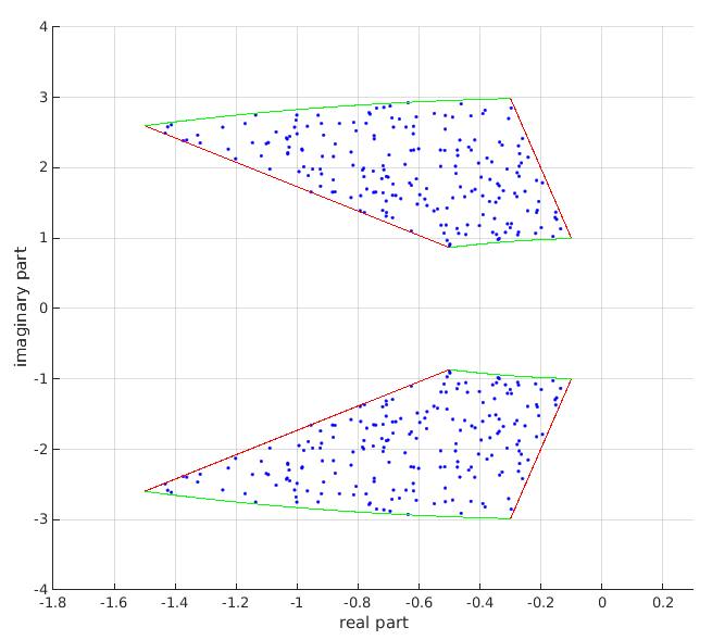
The damping ratio and the frequency lie between the considered bounds in all cases.
The actuator and the 2nd order system are finally connected.
>> sys=sys*actuator;>> size(sys)
Continuous-time GSS object sys with 2 outputs, 1 input and 3 states.
4 blocks in Delta: global size = 5x5.Name Type Size Measured NomValue Boundsposition SAT 1x1 ? 1 limits = [-2 3]damping PAR (real) 1x1 no 0.3 min/max = [0.1 0.5]frequency PAR (real) 2x2 no 2 min/max = [1 3]tau PAR (real) 1x1 no 0 min/max = [-1 1]
PID controller design
A PID controller is now designed using pole placement.
The objective is to design the 1$\times$3 static matrix gain $K$ so that the uncertain closed-loop plant sys behaves like a second-order system with frequency > 1 rad/s and damping > 0.7.
An augmented open-loop plant including an integrator is first computed.
Direct computation
>> Int=gss('Int');>> sysaug1=[-Int 0;1 0;0 1]*sys;
Use of the Simulink library GSSLIB
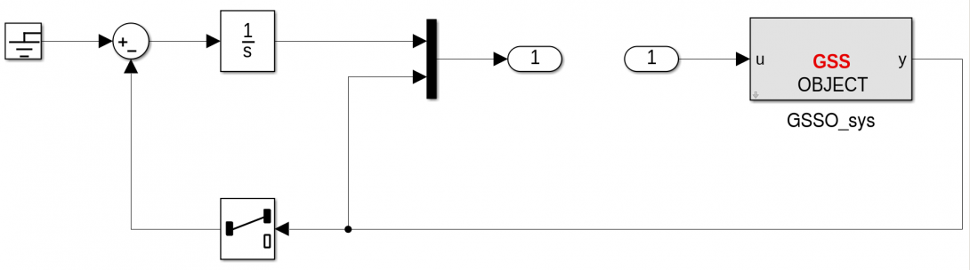
>> sysaug2=slk2gss('open_loop_plant');
Comparison
>> distgss(sysaug1,sysaug2)
$\Rightarrow$ the returned value is zero!
>> sysaug=sysaug1;
An LTI model corresponding to the lowest damping ratio and the lowest frequency is considered for design.
>> syslti=eval(sysaug,{'position' 'tau' 'damping' 'frequency'},{'nominal' 'nominal' 0.1 1});>> damp(syslti)
An eigenstructure assignment algorithm is applied. The main objective is to improve the damping factor, which is set to 0.8.
>> xi_target=0.8;>> omega_target=2;>> lambda=[roots([1 2*xi_target*omega_target omega_target^2]);-2*omega_target];>> for k=1:3>> vw(:,k)=null([syslti.a-lambda(k)*eye(4) syslti.b]);>> end>> K=real(vw(5,:)*inv(syslti.c*vw(1:4,:)));>> damp(syslti.a+syslti.b*K*syslti.c) Pole Damping Frequency Time Constant -4.00e+00 1.00e+00 4.00e+00 2.50e-01-3.00e+00 1.00e+00 3.00e+00 3.33e-01-1.60e+00 + 1.20e+00i 8.00e-01 2.00e+00 6.25e-01-1.60e+00 - 1.20e+00i 8.00e-01 2.00e+00 6.25e-01
The static controller $K=[\begin{array}{ccc}4.80&-5.64&-3.54\end{array}]$ is obtained.
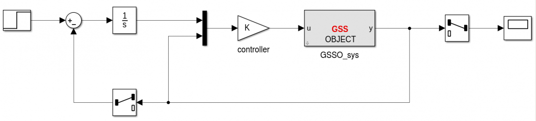
The open-loop model and the controller are interconnected to get the closed-loop plant.
>> syscl=feedback(sysaug,K,[],[],1);
Note that it can also be done using the Simulink library GSSLIB.
The linearized closed-loop plant is analyzed. The saturation is ignored and 200 random samples are computed.
>> syscl_lin=eval(syscl,'position','nominal');>> [sys0,samples]=dbsample(syscl_lin,200);>> syscl_lin=eval(syscl,'position','nominal');>> [sys0,samples]=dbsample(syscl_lin,200);>> for k=1:length(sys0)>> ev=eig(sys0{k});>> plot(real(ev),imag(ev),'m.')>> end>> plot(-0.7*[1 3],sqrt(1-0.7^2)*[1 3],'r-')>> plot(-0.7*[1 3],-sqrt(1-0.7^2)*[1 3],'r-')>> theta=pi-0.795:0.001:pi+0.795;>> plot(cos(theta),sin(theta),'g-')
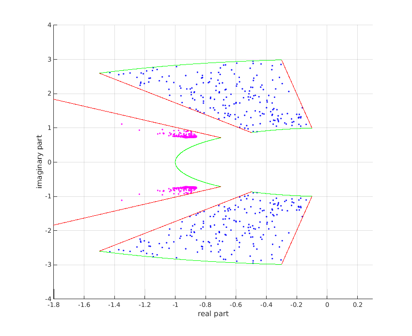
The damping ratio and the frequency lie inside the considered bounds in all cases.
Closed-loop analysis
The nonlinear closed-loop plant is analyzed. A simulation is performed (including the saturation) for each of the 200 random samples computed previously.
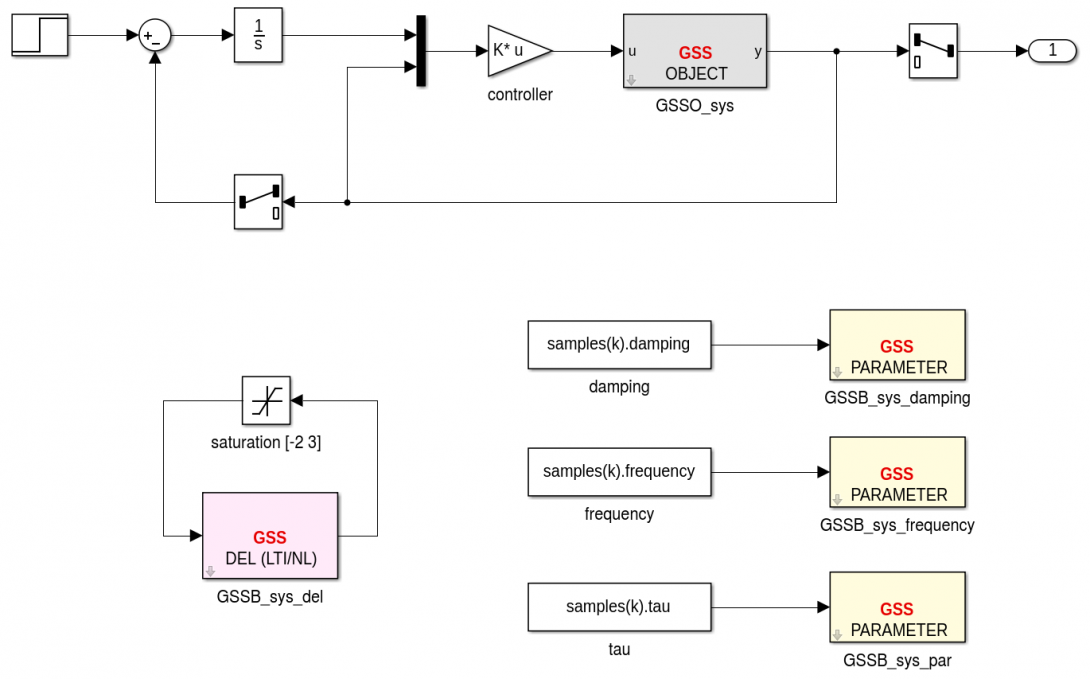
>> figure>> subplot(1,2,1),hold on,grid on>> ref=1;>> for k=1:length(sys0)>> [t,x,y]=sim('closed_loop_plant_uncertain');>> plot(t,y,'b-');>> end>> xlabel('t')>> ylabel('output for reference = 1')>> subplot(1,2,2),hold on,grid on>> ref=3;>> for k=1:length(sys0)>> [t,x,y]=sim('closed_loop_plant_uncertain');>> plot(t,y,'b-');>> end>> xlabel('t')>> ylabel('output for reference = 3')>> subplot(1,3,3),hold on,grid on
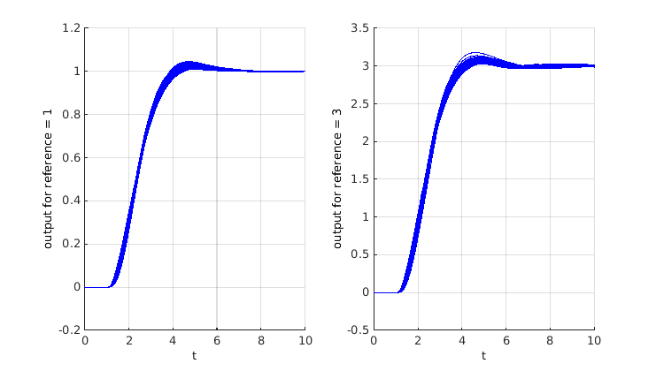
Figure 4: Closed-loop simulations for the 200 random samples
The closed-loop behavior is in accordance with the specifications, but the influence of the saturation can be seen for a reference input of 3.
It seems to work... but further validation is required. This can for example be achieved with other libraries of the SMAC Toolbox (SMART, SAW, IQC).