Please report any problems to Clément Roos (croos@onera.fr). I will try to fix them as quickly as possible!
Overview
The SMART library (Skew Mu Analysis based Robustness Tools) of the SMAC toolbox contains a set of $\mu$-analysis based tools to evaluate the robustness properties of high-dimensional LTI plants subject to numerous LTI uncertainties. These tools allow to compute both upper and lower bounds on the (skewed) robust stability margin, the worst-case $\mathcal{H}_\infty$ performance level, as well as the worst-case gain, phase, modulus and time-delay margins. The key idea is to solve the problem on just a coarse frequency grid and to perform a fast validation on the whole frequency range, which results in guaranteed but conservative bounds on the aforementioned quantities. Some heuristics are then applied to determine a set of worst-case parametric configurations leading to over-optimistic bounds. A branch and bound scheme is finally implemented, so as to tighten these bounds with the desired accuracy, while still guaranteeing a reasonable computational complexity. A short summary of all these algorithms can be found in [1].
Problem statement
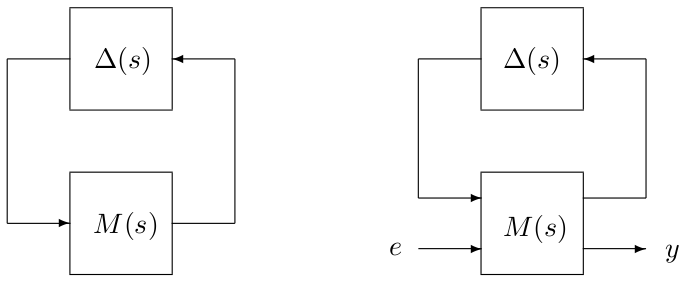
Let us consider the standard interconnections of Figure 1. $M(s)$ is a continuous-time stable and proper real-rational transfer function representing the nominal closed-loop system. $\Delta(s)$ is a continuous-time block-diagonal LTI operator: $$\Delta(s)=\mbox{diag}(\Delta_1(s),\dots,\Delta_N(s))$$ which gathers all model uncertainties. Each $\Delta_i(s)$ can be:
- either a time-invariant diagonal matrix $\Delta_i(s)=\delta_iI_{n_i}$, where $\delta_i$ denotes a real or complex parametric uncertainty,
- or a stable and proper real-rational unstructured transfer function of size $n_i\times n_i$ usually representing neglected dynamics.
Let $n=\sum_{i=1}^{N}n_i$. The set of all $n\times n$ matrices with the same block-diagonal structure and the same nature (real or complex) as $\Delta(j\omega)$ is denoted by $\bf\Delta$. The notation $\Delta(s)\in\bf\Delta$ is then introduced to specify that $\Delta(j\omega)\in\bf\Delta$ for all $\omega\in\Omega$, where $\Omega$ denotes the frequency range of interest (usually equal to $\mathbb{R}_+$). Finally, let $k\mathcal{B}_{{\bf\Delta}}= \{\Delta\in{\bf\Delta}\,:\,\overline{\sigma}(\Delta) < k\}$, where $\overline{\sigma}\left(.\right)$ denotes the largest singular value.
$\mu$-analysis [2] is probably the most efficient technique to analyze the robustness properties of the interconnections of Figure 1, especially when high-dimensional systems are considered. The underlying theory [3,4] is not broached as such in this paper due to space limitations, but a few useful definitions are recalled below.
Definition 1. Let $\omega\in\mathbb{R}_+$ be a given frequency. If no matrix $\Delta\in{\bf\Delta}$ makes $I-M(j\omega)\Delta$ singular, then the structured singular value $\mu_{\bf\Delta}(M(j\omega))$ is equal to zero. Otherwise:
\begin{equation} \mu_{\bf\Delta}(M(j\omega))=\Big[\min_{\Delta\in{\bf\Delta}}\left\{\overline{\sigma}(\Delta),\,\textrm{det}(I-M(j\omega)\Delta)=0\right\}\Big]^{-1} \end{equation}
Lemma 1. The interconnection of Figure 1 (left) is stable $\forall\Delta(s)\in k_r\mathcal{B}_{\bf\Delta}$, where the robust stability margin $k_r$ is defined as the inverse of the largest value of $\mu_{\bf\Delta}(M(j\omega))$ over the frequency range of interest:
\begin{equation} k_r = \Big[\max_{\omega \in\Omega}\,\mu_{\bf\Delta}(M(j\omega))\Big]^{-1} \end{equation}
Assume now that ${\bf\Delta}$ is split into two distinct block structures, i.e. ${\bf\Delta}=\mbox{diag}({\bf\Delta_f},{\bf\Delta_u})$. Let ${\bf\Delta_s}=\mbox{diag}(\mathcal{B}_{\bf\Delta_f},{\bf\Delta_u})$ and $k\mathcal{B}_{\bf\Delta_s}=\mbox{diag}(\mathcal{B}_{\bf\Delta_f},k\mathcal{B}_{\bf\Delta_u})$. The skewed structured singular value is defined as follows [5].
Definition 2. Let $\omega\in\mathbb{R}_+$ be a given frequency. If no matrix $\Delta=\mbox{diag}(\Delta_f,\Delta_u)\in{\bf\Delta_s}$ makes $I-M(j\omega)\Delta$ singular, then the skewed structured singular value $\nu_{\bf\Delta_s}(M(j\omega))$ is equal to zero. Otherwise:
\begin{equation} \nu_{\bf\Delta_s}(M(j\omega))=\Big[\min_{\Delta\in{\bf\Delta_s}}\left\{\overline{\sigma}(\Delta_u),\,\textrm{det}(I-M(j\omega)\Delta)=0\right\}\Big]^{-1} \end{equation}
Lemma 2. The interconnection of Figure 1 (left) is stable $\forall\Delta(s)\in k_s\mathcal{B}_{\bf\Delta_s}$, where the skewed robust stability margin $k_s$ is defined as the inverse of the largest value of $\nu_{\bf\Delta_s}(M(j\omega))$ over the frequency range of interest:
\begin{equation} k_s = \Big[\max_{\omega \in\Omega}\,\nu_{\bf\Delta_s}(M(j\omega))\Big]^{-1} \end{equation}
In other words, $k_s$ is the $H_\infty$ norm of the smallest uncertainty $\Delta_u(s)\in{\bf\Delta_u}$ such that there exists $\Delta_f(s)\in\mathcal{B}_{\bf\Delta_f}$ for which the interconnection between $M(s)$ and $\Delta(s)=\mbox{diag}(\Delta_f(s),\Delta_u(s))\in{\bf\Delta_s}$ is unstable. $\Delta_f(s)$ and $\Delta_u(s)$ thus correspond to fixed range and unbounded uncertainties respectively. $\nu$-analysis is a more general framework than $\mu$-analysis, since the classical structured singular value is recovered in Definition 2 if ${\bf\Delta_f}$ is empty. It also proves to be very useful in practice. Indeed, it allows to consider a wide class of analysis problems, such as computing the worst-case $H_\infty$ performance level, the maximal allowable amount of parametric uncertainties in the presence of neglected dynamics, and the worst-case gain, phase, modulus and delay margins.
The exact computation of $k_r$ or $k_s$ is known to be NP hard in the general case [6], so both lower and upper bounds are computed instead. But even computing these bounds is a challenging problem with an infinite number of frequency-domain constraints. It is usually solved on a finite frequency grid $(\omega_i)_{i\in [1,m]}$ and estimates of the robust stability margins are then obtained as:
\begin{equation*} \frac{1}{\displaystyle\max_{i\in [1,m]}(\overline{\mu}_{\bf\Delta}(M(j\omega_i)))}\le\ k_r\le \frac{1}{\displaystyle\max_{i\in [1,m]}(\underline{\mu}_{\bf\Delta}(M(j\omega_i)))} \end{equation*}
\begin{equation*} \frac{1}{\displaystyle\max_{i\in [1,m]}(\overline{\nu}_{\bf\Delta_s}(M(j\omega_i)))}\le\ k_s\le \frac{1}{\displaystyle\max_{i\in [1,m]}(\underline{\nu}_{\bf\Delta_s}(M(j\omega_i)))} \end{equation*}
where lower and upper bounds $\underline{\mu}_{\bf\Delta}$ and $\overline{\mu}_{\bf\Delta}$ on $\mu_{\bf\Delta}$ at a given frequency $\omega_i$ can be computed using the methods of [7,8] and [9] respectively, while lower and upper bounds $\underline{\nu}_{\bf\Delta_s}$ and $\overline{\nu}_{\bf\Delta_s}$ on $\nu_{\bf\Delta_s}$ at a given frequency $\omega_i$ can be computed using the methods of [10] and [11] respectively.
However, a crucial problem appears in this procedure: the grid must contain the most critical frequency point for which the maximal value of $\mu_{\bf\Delta}$ or $\nu_{\bf\Delta_s}$ is reached. If not, the upper bound on $k_r$ or $k_s$ can be very poor, notably in the case of flexible systems, whose $\mu_{\bf\Delta}$ or $\nu_{\bf\Delta_s}$ plot often exhibits very high and narrow peaks. Even worse, the lower bound can be over-evaluated, i.e. be larger than the real value of $k_r$ or $k_s$. Unfortunately, the aforementioned critical frequency is usually unknown! In this context, the considered frequency grid must be sufficiently dense, which can lead to a prohibitive computational cost. But even so, it is still possible to miss a critical frequency (see for example [12]).
To overcome this issue and compute both tight and reliable bounds on $k_r$ and $k_s$, some efficient methods are implemented in the SMART library of the SMAC toolbox. Their key features are summarized below:
- An upper bound on $\mu_{\bf\Delta}$ or $\nu_{\bf\Delta_s}$ is computed at some frequency, for which nothing has been assessed yet. This bound is slightly increased, and a frequency interval on which it remains valid is computed. Such a strategy is repeated until the whole frequency range is investigated, leading to a lower bound $\underline{k}_r$ or $\underline{k}_s$ on $k_r$ or $k_s$ [13,14]. The latter is guaranteed on the whole frequency range, and not only on a frequency grid as it is the case of most existing methods. See the routines
muubandmuub_mixed. - Some heuristics are applied to determine the smallest possible perturbation $\tilde{\Delta}(s)\in{\bf\Delta}$ or ${\bf\Delta_s}$ such that $\mbox{det}(I-M(j\tilde{\omega})\tilde{\Delta}(j\tilde{\omega}))=0$ for some frequency $\tilde{\omega}\in\Omega$, i.e. such that the interconnection between $M(s)$ and $\tilde{\Delta}(s)$ is unstable. A lower bound on $\mu_{\bf\Delta}$ or $\nu_{\bf\Delta_s}$, and thus an upper bound $\overline{k}_r$ or $\overline{k}_s$ on $k_r$ or $k_s$, is then obtained [15,12]. Unlike most existing methods, frequency is an optimization parameter, which allows to detect critical frequencies and usually leads to more accurate bounds. See the routines
mulb,mulb_mixed,mulb_nreal,mulb_1realandhinflb_real. - A branch and bound algorithm is implemented. It allows to tighten the gap between the bounds on $k_r$ or $k_s$ to the desired accuracy at a reasonable computational cost [1]. The $\mu$-sensitivities are used to select the most critical uncertainties [18,19]. See the routines
mubbandmubb_mixed.
In this context, four main issues can be addressed by the SMART library of the SMAC toolbox:
- robust stability margin - With reference to Figure 1 (left), compute the robust stability margin $k_r$ for a given block structure ${\bf\Delta}$.
- skewed robust stability margin - With reference to Figure 1 (left), compute the skewed robust stability margin $k_s$ for a given block structure ${\bf\Delta_s}$.
- worst-case $\mathcal{H}_\infty$ performance level - With reference to Figure 1 (right) and assuming that $k_r>1$, compute the highest value $k_\infty$ of the $\mathcal{H}_\infty$ norm of the transfer matrix from $e$ to $y$ when $\Delta(s)$ takes all possible values in $\mathcal{B}_{\bf\Delta}$.
- worst-case input-output margins - With reference to Figure 1 (right) and assuming that $k_r>1$, compute the worst-case gain, modulus, phase and delay margins $k_g$, $k_m$, $k_p$ and $k_d$, i.e. the highest value of the (real or complex) gain, the phase shift or the time delay that can be inserted between $y$ and $e$ without destabilizing the system when $\Delta(s)$ takes all possible values in $\mathcal{B}_{\bf\Delta}$.
Both lower and upper bounds on $k_r$, $k_s$, $k_\infty$, $k_g$, $k_m$, $k_p$ and $k_d$ can be computed with the desired accuracy:
- robust stability margin computation is a classical $\mu$ problem, which can be solved by computing lower and upper bounds on $\mu_{\bf\Delta}$ on the whole frequency range,
- skewed robust stability margin, worst-case $\mathcal{H}_\infty$ performance [12] and input-output margins [1,16] computation are skew-$\mu$ (or $\nu$) problems, which can be solved by computing lower and upper bounds on $\nu_{\bf\Delta_s}$ on the whole frequency range.
References
| [1] | C. Roos, F. Lescher, J-M. Biannic, C. Doll and G. Ferreres, "A set of $\mu$-analysis based tools to evaluate the robustness properties of high-dimensional uncertain systems", in Proceedings of the IEEE Multiconference on Systems and Control, Denver, Colorado, September 2011, pp. 644-649. |
| [2] | J. Doyle, "Analysis of feedback systems with structured uncertainties", IEE Proceedings, Part D, vol. 129, no. 6, pp. 242-250, 1982. |
| [3] | G. Ferreres, A practical approach to robustness analysis with aeronautical applications, Springer Verlag, 1999. |
| [4] | K. Zhou, J. Doyle and K. Glover, Robust and optimal control, Prentice-Hall, New Jersey, 1996. |
| [5] | M. Fan and A. Tits, "A measure of worst-case $\mathcal{H}_\infty$ performance and of largest acceptable uncertainty", Systems and Control Letters, vol. 18, no. 6, pp. 409-421, 1992. |
| [6] | R. Braatz, P. Young, J. Doyle and M. Morari, "Computational complexity of $\mu$ calculation", IEEE Transactions on Automatic Control, vol. 39, no. 5, pp. 1000-1002, 1994. |
| [7] | P. Young and J. Doyle, "A lower bound for the mixed $\mu$ problem", IEEE Transactions on Automatic Control, vol. 42, no. 1, pp. 123-128, 1997. |
| [8] | P. Seiler, A. Packard and G. Balas, "A gain-based lower bound algorithm for real and mixed $\mu$ problems", Automatica, vol. 46, no. 3, pp. 493-500, 2010. |
| [9] | P. Young, M. Newlin and J. Doyle, "Computing bounds for the mixed $\mu$ problem", International Journal of Robust and Nonlinear Control, vol. 5, no. 6, pp. 573-590, 1995. |
| [10] | G. Ferreres and V. Fromion, "Robustness analysis using the $\nu$ tool", in Proceedings of the 35th IEEE Conference on Decision and Control, Kobe, Japan, December 1996, pp. 4566-4571. |
| [11] | G. Ferreres and V. Fromion, "Computation of the robustness margin with the skewed $\mu$ tool", Systems and Control Letters, vol. 32, no. 4, pp. 193-202, 1997. |
| [12] | C. Roos, "A practical approach to worst-case $\mathcal{H}_\infty$ performance computation", in Proceedings of the IEEE Multiconference on Systems and Control, Yokohama, Japan, September 2010, pp. 380-385. |
| [13] | C. Roos and J-M. Biannic, "Efficient computation of a guaranteed stability domain for a high-order parameter dependent plant", in Proceedings of the American Control Conference, Baltimore, Maryland, July 2010, pp. 3895-3900. |
| [14] | G. Ferreres, J-F. Magni and J-M. Biannic, "Robustness analysis of flexible structures: practical algorithms", International Journal of Robust and Nonlinear Control, vol. 13, no. 8, pp. 715-734, 2003. |
| [15] | G. Ferreres and J-M. Biannic, "Reliable computation of the robustness margin for a flexible transport aircraft", Control Engineering Practice, vol. 9, pp. 1267-1278, 2001. |
| [16] | F. Lescher and C. Roos, "Robust stability of time-delay systems with structured uncertainties: a $\mu$-analysis based algorithm", in Proceedings of the 50th IEEE Conference on Decision and Control, Orlando, Florida, December 2011, pp. 4955-4960. |
| [17] | J-M. Biannic and G. Ferreres, "Efficient computation of a guaranteed robustness margin", in Proceedings of the 16th IFAC World Congress, Prague, Czech Republic, July 2005. |
| [18] | J. Lesprier, C. Roos and J-M. Biannic, "Improved $\mu$ upper bound computation using the $\mu$-sensitivities", in Proceedings of the 8th IFAC Symposium on Robust Control Design, Bratislava, Slovak Republic, July 2015, pp. 214-219. |
| [19] | R. Braatz and M. Morari, "$\mu$-sensitivities as an aid for robust identification", in Proceedings of the American Control Conference, Boston, Massachusetts, June 1991, pp. 231-236. |