There is something striking with $\mu$ analysis. On the one hand, it appears to be a very mature technique. Several different methods have been developed in the last 30 years in order to tackle the problem of computing the structured singular value $\mu$, and very relevant results are reported in a number of papers. On the other hand, only few well-documented softwares are widely available, and many practical algorithms have only been evaluated by their respective authors. As a result, control engineers and researchers often have to rely on the algorithms implemented in the Robust Control toolbox for Matlab. This observation raizes an important issue: are these tools state-of-the-art or can they be outperformed?
Another difficulty is that the exact computation of $\mu$ is NP hard in the general case, so both lower and upper bounds have to be computed instead. Most of the computationally tractable methods to compute $\mu$ upper bounds rely on the so-called $D$ and $G$ scaling matrices. By contrast, there is no such consensus regarding $\mu$ lower bounds. Indeed, a wide number of very different approaches have been developed, as confirmed by the substantial bibliography detailed below. But these bounds are of little help if the gap with respect to the exact value of $\mu$ is large or if the computational cost is excessive. A good method should thus offer a satisfactory compromise between conservatism and CPU time.
In this context, all practical algorithms to compute lower bounds on the structured singular value $\mu$ (i.e. upper bounds on the robust stability margin $k_r$) are evaluated here on a wide set of real-world applications. This is probably the best way to highlight the most promising tools from an engineering perspective, but also to propose appropriate improvements and combinations to get the most out of them. The ultimate goal is of course to bridge the gap between the real value of $\mu$ and its bounds. Another ambition of this work is to provide control engineers with a well-documented software, which can be used without mastering all the underlying theory. In this perspective, new and efficient implementations of the most relevant algorithms and strategies are available in the Skew Mu Analysis based Robustness Tools (SMART) library of the SMAC toolbox, which is currently developed by ONERA (The French Aerospace Lab).
| The main conclusions of this work are summarized below: | |
| $\Rightarrow$ | The poles migration technique of Ferreres and Biannic [1] is the most efficient method for problems with purely real uncertainties. It is implemented in the routine mulb_nreal. |
| $\Rightarrow$ | The power algorithm of Young and Doyle [2] is the most efficient method for problems with purely complex or mixed real/complex uncertainties. It is implemented in the routine mulb_mixed. |
| $\Rightarrow$ | Both methods provide very accurate results with very low computational time. |
All numerical data related to the benchmarks can be downloaded here. Each benchmark is described either by an uncertain state-space model usys, or by standard matrices sys and blk which can be directly passed to low-level routines such as mussv, mulb_nreal or mulb_mixed. Both descriptions are of course equivalent and can be used with Matlab R2012b or higher.
This page is organized as follows. All approaches to compute lower bounds on the structured singular value are first surveyed. Detailed numerical results are then presented and analyzed. An extension to skew-μ lower bound computation is finally proposed.
Exhaustive survey of $\mu$ lower bound algorithms
All methods that can reasonably be applied to real-world benchmarks are mentioned. Only a few exponential-time algorithms are omitted, as well as techniques with a very limited range of application. In all cases, both $\mu$ lower bounds and associated destabilizing values of the uncertainties are obtained. For most methods, frequency is fixed during optimization. In this case, $M(j\omega)$ and $\Delta(j\omega)$ are constant matrices, which are simply denoted by $M$ and $\Delta$.
1. Exponential-time methods
The first methods to compute $\mu$ lower bounds were proposed in the 1980's and most of them are exponential-time. One of the best known was introduced in [3] for non-repeated ($n_i=1$) real uncertainties and later generalized in [4,5,6]. It uses the mapping theorem of [7]: the image of $k\mathcal{B}_{{\bf\Delta}}$ by the operator $\Delta\rightarrow\textrm{det}(I-\Delta M)$ is included into the convex hull of the images of the $2^N$ vertices of $k\mathcal{B}_{{\bf\Delta}}$. A $\mu$ lower bound is obtained by considering the position of these images with respect to the origin in the complex plane. Like the mapping theorem, the Kharitonov's theorem [8] and the edge theorem [9] can also be interpreted in a frequency domain approach and used to derive $\mu$ lower bound algorithms. These are not detailed here, but a few interesting references can be found in [5,6].
Then, the algebraic method proposed in [10] for non-repeated real uncertainties searches for a destabilizing uncertainty $\Delta \in k \mathcal{B}_\mathbf{\Delta}$ such that all the $\delta_i$ except 2 attain the maximal magnitude $k$, which can be achieved by simple matrix algebra operations. A one-dimensional halving search on $k$ is performed to compute a $\mu$ lower bound. There are $N(N-1)/2$ ways to choose $2$ uncertainties among $N$ and $2^{N-2}$ ways to set each of the $N-2$ others to $-k$ or $k$, so $N(N-1)2^{N-3}$ searches are performed for each value of $k$. The method presented in [11] is quite similar. It is based on the computation of the smallest common real root of a system of linear polynomials using the Sylvester's theorem [12]. The main difference with [10] is that both $k$ and the two $\delta_i$ which do not attain the maximal magnitude are computed in a single step. The optimal value of $k$ is thus determined directly and no halving search is required.
More recently, a method was presented in [13] for (possibly repeated) real uncertainties. It consists of introducing $b=\prod_{i=1}^{N}(n_i+1)-1$ fictitious uncertainties $\overline{\delta}_1,\dots,\overline{\delta}_b$ and rewriting the numerator of $\textrm{det}(I-M(s)\Delta)$ as $f(s)=\hat{p}(s)+\left[\,\overline{\delta}_1\dots\overline{\delta}_b\right] \left[p_1(s)\dots p_b(s)\right]^T$, where $\hat{p}(s),p_1(s),\dots,p_b(s)$ are fixed real polynomials. The stability of $f(s)$ is then evaluated using the stability feeler introduced in [14], which leads to $\mu$ upper and lower bounds.
The algorithms mentioned in this section have different theoretical foundations. But they are all exponential-time, which means that they cannot be applied to most real-world benchmarks with a reasonable computational time. Thus, only polynomial-time algorithms are considered in the sequel.
2. Power algorithm
This technique can be used for all kinds of uncertainties. It is based on the following characterization [2]:
| \begin{equation}\mu_{\bf\Delta}(M)=\max_{Q\in\mathcal{Q}}\rho_R(QM)\end{equation} | (1) |
where $\rho_R(QM)$ is the largest magnitude of the real eigenvalues of $QM$, while $\mathcal{Q}$ is the set of all $\Delta=\textrm{diag}(\Delta_1,\dots,\Delta_N)\in{\bf\Delta}$ such that $\delta_i\in [-1,1]$ if $\Delta_i=\delta_iI_{n_i}$ is real and $\Delta_i^*\Delta_i=I_{n_i}$ if $\Delta_i$ is complex. Equation (1) defines a non-concave optimization problem, which is solved in [2] using a fixed point iteration usually referred to as the power algorithm. No theoretical convergence guarantee exists. But if the algorithm converges, a local maximum, i.e. a $\mu$ lower bound, is obtained. In practice, convergence is usually ensured for purely complex and mixed real/complex uncertainties. But in the purely real case, limit cycles often appear and no $\mu$ lower bound can be obtained. Nevertheless, a technique is proposed in [15] to get a nontrivial $\mu$ lower bound when the power algorithm does not converge but returns nonzero values. Further improvements are also reported in [16,17,18].
A different way to solve problem (1) is proposed in [19] in the particular case of purely complex uncertainties ($\rho_R$ is then replaced with the spectral radius $\rho$). The steepest ascent and the conjugate gradient algorithms are used instead of a fixed-point iteration. Unlike the power algorithm, which only provides a $\mu$ lower bound in case of convergence, a nontrivial bound is obtained at each iteration at the price of a higher computational cost.
3. Gain-based algorithm
This method was introduced in [20] to address the convergence issues of the power algorithm when purely real uncertainties are considered. The initial $\mu$ problem is replaced with a series of worst-case $H_\infty$ performance problems, which are efficiently solved using the approach of [21]. In the mixed real/complex case, the real blocks of the destabilizing uncertainties are obtained using the aforementioned technique, while the complex blocks are computed using the power algorithm.
4. Poles migration techniques
These techniques are mainly dedicated to purely real problems, although they can in some cases be extended to handle mixed and complex uncertainties. The idea is to move an eigenvalue of the interconnection between $M(s)$ and $\Delta$ towards the imaginary axis, which requires to work in the time domain. The state matrix of the interconnection is $A_0=A+B\Delta(I-D\Delta)^{-1}C$, where $(A,B,C,D)$ is a state-space representation of $M(s)$. An equivalent definition of the structured singular value can thus be derived:
\begin{equation} \mu_{\bf\Delta}(M(j\omega)) = \Big[\min_{\Delta\in{\bf\Delta}}\left\{\overline{\sigma}(\Delta),\,\lambda_{max}(A_0)=0\right\}\Big]^{-1} \end{equation}
where $\lambda_{max}(A_0)=\displaystyle\max_i\,\Re\left(\lambda_i(A_0)\right)$ and $\lambda_i(A_0)$ denotes the $ith$ eigenvalue of $A_0$.
A first approach is to use a first-order characterization of the variation $d\lambda_i$ of $\lambda_i(A_0)$ caused by a small variation $d\Delta$ of $\Delta$. This can be expressed as $d\lambda_i=(uB+tD)d\Delta (Cv+Dw)$, where $u$/$v$ are the left/right eigenvectors associated to $\lambda_i(A_0)$, $t=uB\Delta(I-D\Delta)^{-1}$ and $w=\Delta(I-D\Delta)^{-1}Cv$. A series of perturbations $d\Delta$ are computed, which progressively move the eigenvalues of $A_0$ towards the imaginary axis. Two algorithms exist. On the one hand, a series of quadratic programming problems are solved in [22] for each $\lambda_i(A_0)$. The uncertainty with minimum Froebenius norm which brings $\lambda_i(A_0)$ on the imaginary axis is first determined, and then the one with minimum $\overline{\sigma}$ norm such that the interconnection remains at the limit of stability. On the other hand, [1] notes that the power algorithm of [2] is quite fast, but often suffers from convergence problems when purely real uncertainties are considered. A three-step procedure is proposed in this case. The initial problem is first regularized by adding a small amount $\epsilon\ll 1$ of complex uncertainty, i.e. $\Delta$ is replaced with $\Delta+\epsilon\Delta_C$, where $\Delta_C$ has the same structure as $\Delta$ but can take on complex values [23]. The power algorithm is then run at each point of a rough frequency grid, usually with good convergence properties. Using the resulting uncertainties as an initialization, a series or linear programming problems are finally solved, so as to find the value $\hat{\Delta}$ of $\Delta$ with minimum $\overline{\sigma}$ norm for which one of the eigenvalues of the initial interconnection becomes unstable. The resulting $\mu$ lower bound is equal to $\overline{\sigma}(\hat{\Delta})^{-1}$.
More recently, a direct approach has been proposed by [24,25]. It considers the optimization problem:
| \begin{equation}\min_{\Delta\in{\bf\Delta}}\overline{\sigma}(\Delta)\ \ \textrm{such that}\ \ \lambda_{max}(A_0)=0\end{equation} | (2) |
which can be recast as a sequential quadratic programming problem and solved for example using the Matlab Optimization toolbox. In practice, a relaxed condition is considered to avoid convergence issues: the equality constraint is replaced with $|\lambda_{max}(A_0)|\le\epsilon$, where $\epsilon$ is a small user-defined threshold. Problem (2) is non-convex and the result thus strongly depends on the initial value of $\Delta$. Several strategies are combined in [24] to improve the resulting $\mu$ lower bounds.
5. Optimization-based techniques
These algorithms are directly inspired by the definition of $\mu$. A first approach consists of directly solving the following non-convex optimization problem using standard nonlinear optimization tools such as the fmincon function of the Matlab Optimization toolbox:
| \begin{equation}\min_{\Delta\in{\bf\Delta}}\overline{\sigma}(\Delta)\ \ \textrm{such that}\ \ \textrm{det}(I-M\Delta)=0\end{equation} | (3) |
In practice, a relaxed condition is considered to avoid convergence issues: the equality constraint is replaced with $\underline{\sigma}(I-M\Delta)\le\epsilon$ in [26,27], and with $|\textrm{det}(I-M\Delta)|\le\epsilon$ in [28], where $\epsilon$ is a small user-defined threshold. Any kind of uncertainties can be considered, but this approach is especially relevant for purely real problems, since the number of decision variables significantly increases when complex uncertainties are considered.
A formulation similar to (3) is considered in [29] in the case of (possibly repeated) real uncertainties:
\begin{equation} \min_{\scriptsize\begin{array}{c}\Delta\hspace{-0.8mm}\in\hspace{-0.8mm}{\bf\Delta}\\[-3pt]\lambda_1\hspace{-0.3mm},\hspace{-0.3mm}\lambda_2\hspace{-0.6mm}\in\hspace{-0.3mm}\mathbb{R}\end{array}}\overline{\sigma}(\Delta)+(\lambda_1^q+\lambda_2^q)\lambda\ \ \ \textrm{such that}\ \ \left\{\hspace{-1mm}\begin{array}{ll} \Re (\textrm{det}(I-M\Delta))=\lambda_1^p\\\Im (\textrm{det}(I-M\Delta))=\lambda_2^p \end{array}\right. \end{equation}
where $p$ and $q$ are odd and even positive integers respectively, and $\lambda$ is a large penalty parameter. This optimization problem is solved using the modified subgradient algorithm based on feasible values (F-MSG) introduced in [30].
Another variation is proposed in [31]. The following optimization problem is first solved for different values of $k$ using the fmincon function of the Matlab Optimization toolbox:
\begin{equation} g(k)=\min_{\Delta\in k\mathcal{B}_{{\bf\Delta}}}\Re\left(\textrm{det}(I-M\Delta)\right)\ \ \ \textrm{such that}\ \ \ |\Im\left(\textrm{det}(I-M\Delta)\right)|\le\epsilon \end{equation}
where $\epsilon$ is a user-defined threshold. A function $g$ is thus defined. A modification of the Newton-Raphson method called the secant method is then applied to determine the smallest value $\underline{k}$ of $k$ such that $g(k)=0$. A $\mu$ lower bound is finally obtained as the inverse of $\underline{k}$.
A common feature of the aforementioned optimization-based algorithms is that they all use standard nonlinear optimization tools, although the objective to be minimized is a nonsmooth function. Breakdowns might thus be encountered at points that are not local optima, because the latter are typically nonsmooth points in practice. In this context, [32] proposes a nonsmooth optimization technique to solve problem (3), whose convergence to a local minimum is ensured.
6. Geometrical approach
This method dedicated to (possibly repeated) real uncertainties combines randomization and nonlinear optimization [33]. The signs of the real and the imaginary parts of $\textrm{det}(I-M\Delta)$ are computed for randomly selected points on the surface of a given hyperbox in the uncertainty space $\mathbb{R}^N$. This hyperbox is enlarged until the four possible sign combinations are found, which means that it might contain values of $\delta_1,\dots,\delta_N$ such that $\textrm{det}(I-M\Delta)=0$. A series of contractions and expansions are then performed to approach the singular region until the size of the box becomes smaller than some tolerance value.
Remark 1. Except for the poles migration techniques, a classical strategy is to compute $\mu$ lower bounds on a predefined frequency grid. An alternative is to compute bounds on a set of frequency intervals whose union covers the whole frequency range. This can be achieved by considering frequency as an additional uncertainty $\delta_\omega$. An augmented interconnection $\tilde{M}-\tilde{\Delta}$ is obtained, where $\tilde{\Delta}=\textrm{diag}(\Delta,\delta_\omega I_m)$, $m$ is the state dimension of $M(s)$, and the frequency interval of interest is covered when $\delta_\omega\in\mathbb{R}$ varies between $-1$ and $1$ (see e.g. [28,32]). A skew-$\mu$ problem is then to be solved, since $\delta_\omega$ is bounded.
$\mu$ upper bound algorithms
Most of the algorithms which can reasonably be applied to real-world benchmarks are based on the following result [15]:
Theorem 1. Let $\beta>0$. If there exist matrices $D \in {\cal D}$ and $G \in {\cal G}$ which satisfy one of the following relations:
\begin{equation} M^*DM+j(GM-M^*G)\leq \beta^2D \end{equation} \begin{equation} \overline{\sigma}\left((I+G^2)^{-\frac{1}{4}}\left(\frac{DMD^{-1}}{\beta}-jG \right)(I+G^2)^{-\frac{1}{4}}\right)\leq 1 \ \end{equation}
where $\mathcal{D} = \{ D=D^*>0:\forall \Delta\in{\bf\Delta},\,D\Delta = \Delta D\}$ and $\mathcal{G} = \{ G=G^*:\forall \Delta\in{\bf\Delta},\,G\Delta = \Delta^* G \}$, then $\mu_{\bf\Delta}(M) \leq \beta$. The problem of minimizing $\beta$ can be solved either optimally using an LMI solver or faster but suboptimally using a gradient descent algorithm.
Computing an upper bound on $\mu_{\bf\Delta}(M(j\omega))$ on the whole frequency range of interest $\Omega$ is thus a challenging problem with an infinite number of frequency-domain constraints and optimization variables, since Theorem 1 must be applied for each $\omega\in\Omega$. In practice, it is usually solved on a finite frequency grid only (see e.g. the function mussv of the Matlab Robust Control toolbox). However, a crucial problem appears in this procedure: the grid must contain the most critical frequency point for which the maximal value of $\mu_{\bf\Delta}(M(j\omega))$ is reached. If not, the resulting lower bound on $k_r$ can be over-evaluated, i.e. be larger than the real value of $k_r$. Unfortunately, the aforementioned critical frequency is usually unknown! To overcome this issue, several approaches have been proposed to compute $\mu$ upper bounds which are guaranteed on the whole frequency range (see e.g. [34,35,36,37,38]). Most of them first use the characterizations of Theorem 1 to compute bounds at given frequencies. A hamiltonian-based technique is then implemented to determine the frequency intervals on which these bounds remain valid. A guaranteed $\mu$ upper bound is finally obtained as soon as the union of all intervals covers the whole frequency range of interest.
Several other techniques exist to compute $\mu$ upper bounds (see e.g. [3,39,40,41]) Nevertheless, they usually require a very high computational time when realistic applications are considered, so they are not detailed here. Note also that the above enumeration is not exhaustive, since this page mainly focuses on $\mu$ lower bound algorithms.
Testing framework
Considered algorithms
The most relevant lower bound algorithms are summarized in Table 1 and compared below. The first two are implemented in the function mussv of the standard Matlab Robust Control toolbox, which is called with the optional argument 'f' and 'fg' respectively. The fourth one is implemented in the function mulb_nreal of the SMART library and is used with default values of the optional parameters. It is based on a function already available in the Skew Mu toolbox for Matlab [42], which has been improved in [43]. For the other five algorithms, Matlab functions provided by the respective authors are used, with default values of the optional parameters in most cases (some slight modifications have been performed to handle the trade-off between accuracy and computational time). It is worth being emphasized that each of the eight considered algorithms is called in a similar fashion for all benchmarks.
| Description | Reference | Admissible uncertainties | |
| 1 | Power algorithm | [2] | all |
| 2 | Gain-based algorithm | [20] | real and mixed real/complex |
| 3 | Poles migration technique | [22] | all |
| 4 | Poles migration technique | [1] | real |
| 5 | Poles migration technique | [24] | all |
| 6 | Direct nonlinear optimization | [28] | all |
| 7 | Direct nonsmooth optimization | [32] | all |
| 8 | Geometrical approach | [33] | real |
Grid-based methods (1-2-6-7-8) are applied at each point of a 100-point frequency grid generated with the function gen_grid of the SMART library of the SMAC toolbox [43]. This grid is composed of 50 logarithmically-spaced points within the system bandwidth, and 50 additional points used to refine the grid in some frequency regions corresponding to weakly damped modes. Interval-based implementations are available for methods 6 and 7 (see Remark 1). For these algorithms, the system bandwidth is divided into 6 and 4 frequency intervals of equal size on a logarithmic scale respectively. A coarse 10-point frequency grid generated using the function gen_grid is used for method 4. Finally, methods 3 and 5 do not require any frequency grid.
Some $\mu$ lower bound algorithms mentioned in the above survey are not considered in the sequel. First, the exponential-time methods cannot be applied to all benchmarks with a reasonable computational time, so only polynomial-time algorithms are compared. Then, the optimization-based technique of [19] has a very limited range of application and is omitted, since it can only be applied to complex uncertainties. Moreover, [18] shows that the power algorithm is usually more efficient to solve (1) in terms of accuracy and computational time. Finally, the approaches of [29,31] are very similar to the one of [26,27,28] which is already included in the comparison.
Note also that some techniques could be used in addition to any of the lower bound algorithms : the $\mu$-sensitivities introduced in [44] allow to reduce the number of uncertainties and thus the computational time at the price of a loss of accuracy, while branch-and-bound schemes [45] allow to tighten the gap between $\mu$ upper and lower bounds at the price of an increase in the computational time. These techniques are not considered here.
For each benchmark, a $\mu$ upper bound is computed using the algorithm proposed in [34], improved in [35,36] and implemented in the SMART library [43]. It provides an upper bound on the gap between the true value of $k_r$ and the best $k_r$ upper bound obtained with the $\mu$ lower bound algorithms listed in Table 1.
List of benchmarks
As shown in Table 2, a total of 36 challenging benchmarks are considered in this work, corresponding to various fields of application, system dimensions and structures of the uncertainties. Some of them contain poorly damped modes, which usually produce extremely sharp peaks on the $\mu$ plot, while others are characterized by large state vectors as well as numerous and/or highly repeated uncertainties. Purely real uncertainties are majority (benchmarks 1-29), since they are more common in engineering problems than complex or mixed ones (benchmarks 30-36). Moreover, the presence of complex uncertainties usually simplifies the computation of $\mu$ upper and lower bounds, making them of less interest in the present study.
| Description | Reference | States | Size of Δ | Structure of Δ | |
| 1 | Academic example | [46] | 5 | 1 | 1×1 |
| 2 | Academic example | [3] | 4 | 3 | 3×1 |
| 3 | Academic example | [13] | 4 | 4 | 2×2 |
| 4 | Inverted pendulum | [29] | 4 | 3 | 3×1 |
| 5 | Anti-aliasing filter | [20] | 2 | 5 | 3×1 + 1×2 |
| 6 | DC motor | [47] | 4 | 5 | 3×1 + 1×2 |
| 7 | Bus steering system | [48] | 9 | 5 | 1×2 + 1×3 |
| 8 | Satellite | [49] | 9 | 4 | 2×1 + 1×2 |
| 9 | Bank-to-turn missile | [50] | 6 | 4 | 4×1 |
| 10 | Aeronautical vehicle | [51] | 8 | 4 | 4×1 |
| 11 | Four-tank system | [52] | 10 | 4 | 4×1 |
| 12 | Re-entry vehicle | [53] | 6 | 8 | 1×2 + 2×3 |
| 13 | Missile | [54] | 14 | 4 | 4×1 |
| 14 | Cassini spacecraft | [40] | 17 | 4 | 4×1 |
| 15 | Mass-spring-damper system | [55] | 7 | 6 | 6×1 |
| 16 | Spark ignition engine | [56] | 4 | 7 | 7×1 |
| 17 | Hydraulic servo system | [57] | 8 | 8 | 8×1 |
| 18 | Academic example | [58] | 41 | 5 | 3×1 + 1×2 |
| 19 | Drive-by-wire vehicle | [28] | 4 | 16 | 2×1 + 7×2 |
| 20 | Re-entry vehicle | [49] | 7 | 13 | 3×1 + 1×4 + 1×6 |
| 21 | Space shuttle | [59] | 34 | 9 | 9×1 |
| 22 | Rigid aircraft | [54] | 9 | 14 | 14×1 |
| 23 | Fighter aircraft | [49] | 10 | 27 | 7×1 + 1×2 + 1×3 + 1×15 |
| 24 | Flexible aircraft | [54] | 46 | 20 | 20×1 |
| 25 | Telescope mockup | [54] | 70 | 20 | 20×1 |
| 26 | Hard disk drive | [60] | 29 | 27 | 19×1 + 4×2 |
| 27 | Launcher | [49] | 30 | 45 | 16×1 + 10×2 + 1×3 + 1×6 |
| 28 | Helicopter | [61] | 12 | 120 | 4×30 |
| 29 | Biochemical network | [33] | 7 | 507 | 13×39 |
| 30 | Himat fighter aircraft | [59] | 16 | 4 | 2×2(c) |
| 31 | F14 fighter aircraft | [59] | 52 | 8 | 1×2(c) + 1×6(c) |
| 32 | DC motor | [47] | 4 | 6 | 3×1 + 1×2 + 1×1(c) |
| 33 | Four-tank system | [52] | 12 | 6 | 4×1 + 1×2(c) |
| 34 | Missile | [54] | 19 | 6 | 4×1 + 2×1(c) |
| 35 | Hydraulic servo system | [57] | 9 | 9 | 8×1 + 1×1(c) |
| 36 | Space shuttle | [59] | 46 | 18 | 9×1 + 1×9(c) |
Detailed numerical results
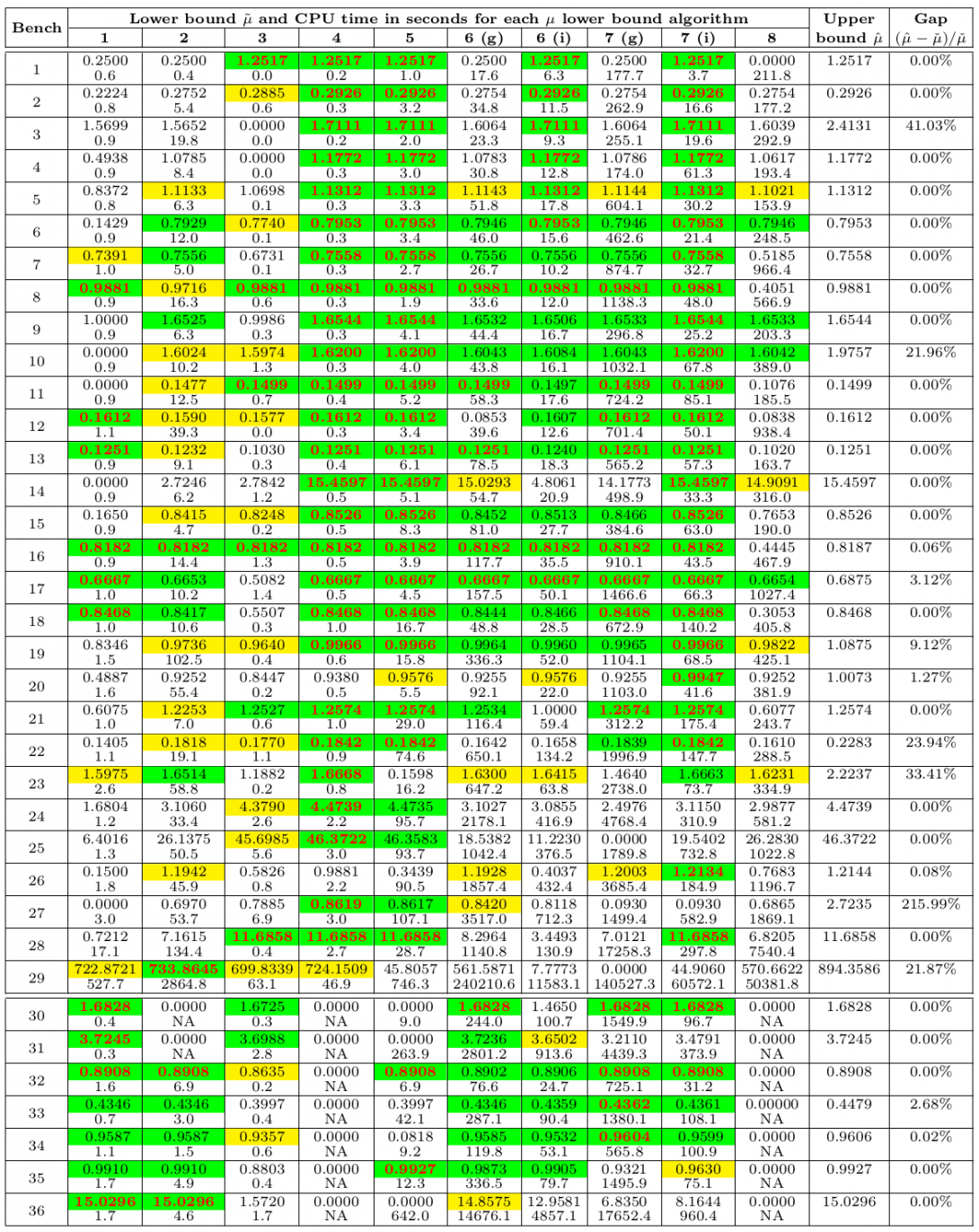
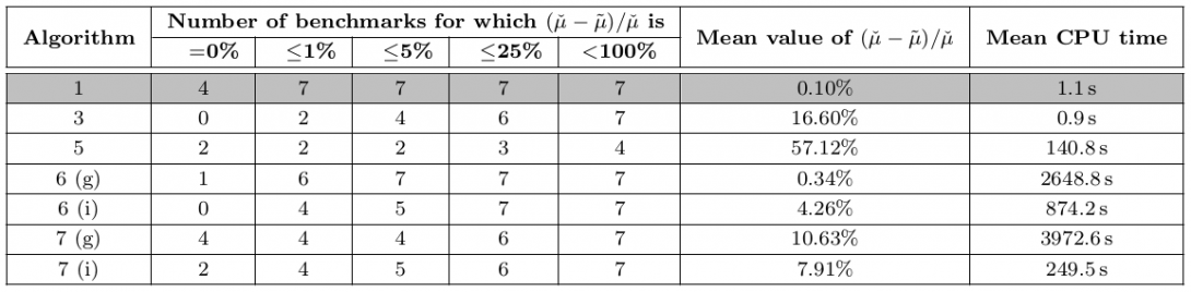
Computations are performed using Matlab R2010b on a Windows 7 Workstation with a CPU Intel Xenon W3530 running at 2.8 GHz and 6 GB of RAM. All results are shown in Table 3. Two lines are used for each benchmark to display first the lower bounds $\tilde{\mu}$ and then the corresponding computational times in seconds. A lower bound $\tilde{\mu}$ is considered to be valid if a frequency $\tilde{\omega}$ and a perturbation $\tilde{\Delta}$ of norm $\tilde{\mu}^{-1}$ are found, which satisfy $|\textrm{det}(I-M(j\tilde{\omega})\tilde{\Delta})|<10^{-8}$. The highest lower bound $\check{\mu}$ out of all algorithms is displayed in red. Bounds which are less than 1% and 5% lower than $\check{\mu}$ are highlighted in green and yellow respectively. NA means that the considered algorithm is not applicable. The symbols (g) and (i) denote the grid-based and the interval-based versions of the algorithms respectively. Finally, the gap between $\check{\mu}$ and the upper bound $\hat{\mu}$ is computed as $(\hat{\mu}-\check{\mu})/\check{\mu}$.
Analysis of the results
Purely real problems
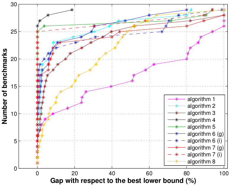
All algorithms are applied to benchmarks 1-29. In Table 4, the mean computational time is computed for each algorithm over all benchmarks except the biochemical network (benchmark 29), which is significantly more complicated than the others and requires a high computational effort. Figure 1 must be interpreted as follows. Let $(x,y)$ be the coordinates of any star sign. Then $y$ corresponds to the number of benchmarks for which the gap $(\check{\mu}-\tilde{\mu})/\check{\mu}$ (upper plot) or the computational time (lower plot) is lower than $x$.
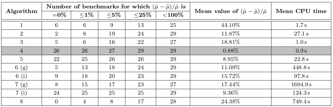
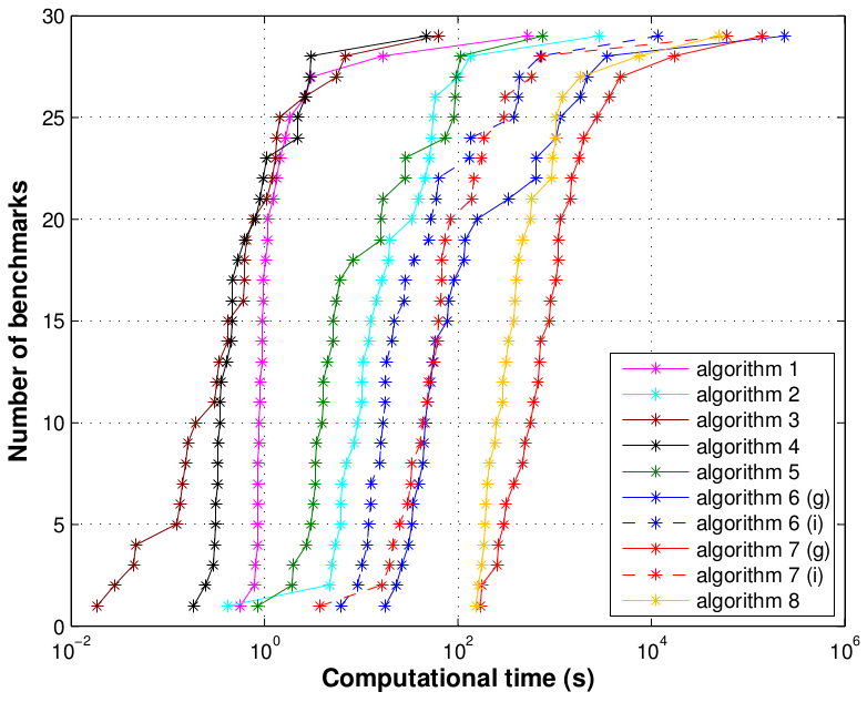
The most relevant algorithm is the poles migration technique of [1], with by far the highest accuracy (less than 1% on average for all 29 benchmarks) and also the lowest computational time (less than 1 second on average for benchmarks 1-28 and 47 seconds for the biochemical network). The poles migration technique of [30] gives very good results too for all except 3 benchmarks, and the computational time remains reasonable (but still 20 times higher). This shows that poles migration is probably the most efficient way to compute accurate $\mu$ lower bounds for purely real problems. Moreover, an attractive feature of this approach is that frequency is not fixed, which allows to detect critical frequencies corresponding to peak values of $\mu$ more easily. The gain-based algorithm of [20], the direct nonlinear optimization technique (grid-based version) of [28] and the direct nonsmooth optimization technique (interval-based version) of [32] also give quite satisfactory results in most cases, since the accuracy is about 10% on average. Nevertheless, these algorithms are much slower (especially the last two). Note also that the nonsmooth technique gives the best results in most cases but sometimes proves very conservative, whereas the nonlinear one usually produces bounds which are not the best ones but yet good ones. Moreover, interval-based versions allow to drastically reduce the computational time, but do not bring any significant improvement in terms of accuracy. Then, the poles migration technique of [22] exhibits both a reasonable accuracy (less than 20% on average for all 29 benchmarks) and a very low computational time (about 1.0 seconds on average for benchmarks 1-28 and only 63 seconds for the biochemical network). Finally, the power algorithm of [2] often suffers from convergence problems, especially for frequencies corresponding to peak values of $\mu_{\bf\Delta}(M(j\omega))$. This is in stark contrast to the complex and mixed cases for which the convergence properties are excellent.
Remark 2. The gain-based algorithm of [20], the direct optimization-based techniques of [28,32] and the geometrical approach of [33] use randomization. Therefore, several runs of these algorithms might provide different $\mu$ lower bounds.
Purely complex and mixed real/complex problems
The poles migration technique of [1] and the geometrical approach of [33] cannot be applied in the presence of complex uncertainties. Moreover, the gain-based algorithm of [20] is not relevant when purely complex uncertainties are considered, since it reduces to the power algorithm of [2], and no improvement over the power algorithm is observed for mixed real/complex problems. Therefore, it is not considered in Table 5 and Figure 2.
The most relevant algorithm is the power algorithm of [2], with the highest accuracy and almost the lowest computational time. This confirms its good convergence properties when mixed or complex uncertaintes are considered. The direct nonlinear optimization technique (grid-based version) of [28] also gives very accurate results, but the mean computational time is 2400 times higher. More generally, optimization-based techniques (algorithms 5-6-7) are not very attractive in terms of computational time, since full complex blocks generate a large number of optimization variables ($2n_i^2$ variables for a $n_i\times n_i$ block).
Approaching the exact value of $\mu$
Purely real problems
The results presented above show that the poles migration technique of [1] is the most relevant method for purely real problems. The best $\mu$ lower bounds are obtained for 26 benchmarks out of 29. Moreover, the bounds computed for the other 3 benchmarks are not very far from the highest values over all algorithms. Improving the poles migration technique to obtain the best results in all cases does not seem to be a trivial issue. Here, the most promising idea is to combine different algorithms to get the most out of them. Apart from the poles migration techniques, the most efficient methods are the gain-based algorithm of [20] and the global optimization tools of [28] and [32]. The following three-step strategy is thus proposed:
- The poles migration technique of [1] (algorithm 4) is executed first.
- The gain-based algorithm of [20] (algorithm 2) is then executed for a few selected frequencies only using the previous results as an initialization. These frequencies can be those for which the uncertain system becomes unstable after algorithm 4 is applied or if a single uncertainty is considered. The frequency for which the lower bound on $k_r$ (i.e. the highest $\mu$ upper bound) is obtained is also a good candidate.
- A global optimization tool such as particle swarm optimization is finally applied using the previous results as an initialization. This kind of techniques offers a bunch of tuning parameters (number of swarms, of particles in each swarm, of topologies...), which allows to easily handle the trade-off between accuracy and computational time.
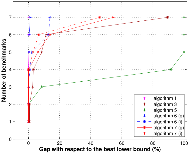
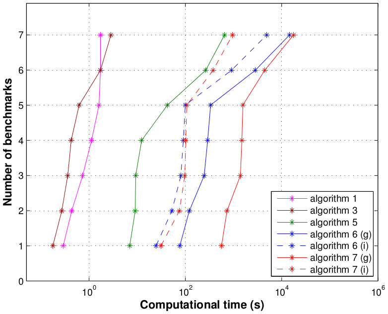
The improved $\mu$ lower bounds so obtained for benchmarks 20/26/29 are shown in Table 6. They are compared with the bounds computed in Table 3 by independently applying all algorithms one at a time.
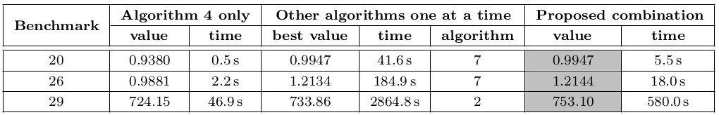
In all cases, the best $\mu$ lower bound is obtained with the proposed strategy. The computational time is of course larger than if algorithm 4 is applied alone. Nevertheless, it remains much smaller than with algorithms 2 and 7, which produced the best results so far. The bound is even improved for benchmarks 26 and 29, for which a single application of any algorithm cannot bring the highest value.
Taking the above results into account, the gap between the best $\mu$ lower bound and the $\mu$ upper bound is 12.71% on average for the 29 purely real problems under consideration. An important issue is now to determine which of the bounds is responsible for this. For 19 benchmarks out of 29, the gap is less than 0.00%. For the other 10, the branch-and-bound algorithm implemented in the function mubb_mixed of the SMART library [62] is applied to improve the $\mu$ upper bound (sometimes with a very high computational cost). Results are presented in Table 7.
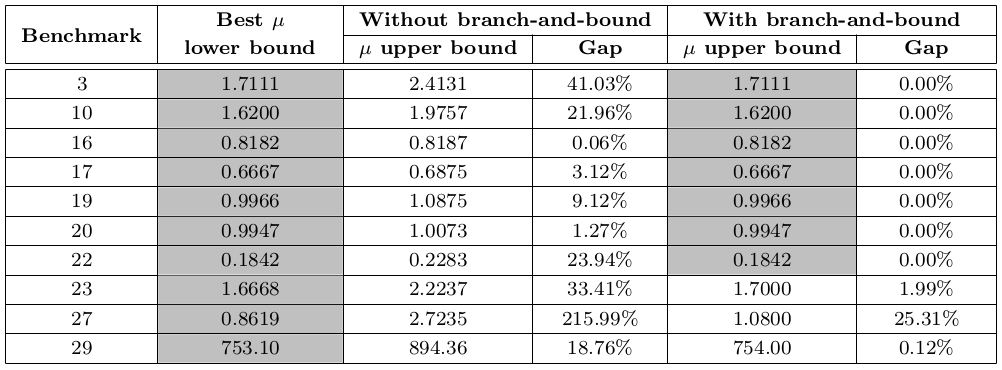
The mean value of the gap over all 29 benchmarks is now only 0.95%. It can thus be concluded that the $\mu$ lower bound computed with the poles migration technique of 4 (eventually combined with the above three-step strategy) almost always equals the exact value of $\mu$. Moreover, the computational time remains very reasonable. This strategy is implemented in the function mulb_nreal of the SMART library.
Purely complex and mixed real/complex problems
The results presented above show that the power algorithm of [2] is the most relevant technique for purely complex and mixed real/complex problems. Nevertheless, the resulting $\mu$ lower bounds are conservative in some cases: the power algorithm is slightly outperformed by other techniques for benchmarks 33/34/35. A careful investigation of several benchmarks including those presented in this page shows that the main reasons for this are threefold:
- The power algorithm is applied at each point of a fixed frequency grid. Unless by some stroke of luck, the critical frequency corresponding to the exact value of $\mu$ is usually not part of this grid, even if the latter is very tight.
- The power algorithm almost always converges in the presence of complex uncertainties, but it sometimes requires a quite large number of iterations.
- Optimization problem (1) is non-concave. Thus, the accuracy of the resulting $\mu$ lower bound strongly depends on the way the power algorithm is initialized.
In this context, the following strategy can be implemented to improve the results displayed in Table 3. First, the power algorithm of [2] is classically applied at each point of a fixed frequency grid. In most cases, the $\mu$ plot does not exhibit very sharp peaks in the presence of complex uncertainties. Thus, a reasonably rough grid (e.g. 20 frequency points) is usually enough to capture approximately the main peaks. Then, the grid is gradually tightened around the frequencies of these peaks until improvement in the $\mu$ lower bound becomes marginal. This strategy allows to address the first two issues highlighted before. Indeed, the grid becomes very tight in the most critical frequency regions and the frequency corresponding to the exact value of $\mu$ can be detected with a very good accuracy. Moreover, repeteadly applying the power algorithm with a limited number of iterations (e.g. 100 iterations) at very close frequencies is roughly equivalent to applying it once with a large number of iterations, provided that it is initialized every time with the result obtained at the previous frequency. Finally, in order to address the third issue, the power algorithm is not only applied with the latter initialization, but also with one or more random initializations at each considered frequency.
The improved $\mu$ lower bounds so obtained for benchmarks 30-36 are shown in Table 8. They are compared with the ones computed by applying the standard power algorithm of the function mussv of the Robust Control toolbox on a fixed frequency grid. The $\mu$ upper bounds are the same as in Table 3 except for benchmark 33, where the branch-and-bound algorithm implemented in the function mubb_mixed of the SMART library has been used to reduce conservatism.
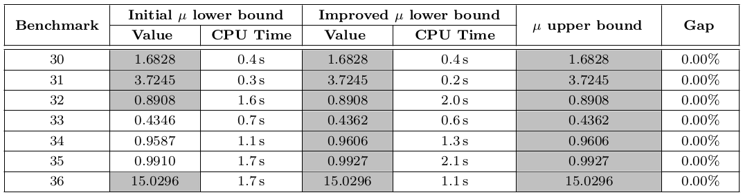
The exact value of $\mu$ is obtained in all cases. The mean computational time is 1.1s. It is exactly the same as with mussv (see Table 5). Indeed, the initial frequency grid is quite rough and it is only tightened in a few selected frequency intervals. Moreover, the number of power iterations performed at each frequency is quite low. The total computational time thus remains very reasonable. The improved version of the power algorithm is implemented in the function mulb_mixed of the SMART library.
Remark 3. Several techniques have been proposed to improve the convergence properties of the power algorithm in case of purely real problems [16,17,18]. But convergence is usually not an issue in the presence of complex uncertainties. These techniques are thus of little help in the present context.
Extension to skew-$\mu$ lower bound computation
Let us now focus on the computation of $k_s$ upper bounds, i.e. of skew-$\mu$ lower bounds (see this page for more details). Most of the $\mu$ lower bound algorithms can be extended more or less easily to handle skew uncertainties. The objective here is not to study these generalizations in details, but to show that the most relevant methods highlighted above still perform very well in the skew case.
Purely complex and mixed real/complex problems
The most efficient $\mu$ lower bound algorithm is by far the power algorithm of [2]. It can be easily extended as explained in [63,64,65]. Combined with the strategy detailed in the previous section, it usually provides very good $\nu$ lower bounds. Indeed, a significant number of tests have revealed that the exact value of $\nu$ can be obtained in many cases. This improved version of the power algorithm is implemented in the function mulb_mixed of the SMART library.
Purely real problems
The most efficient $\mu$ lower bound algorithm is the poles migration technique of [1]. It can be easily extended to skew-$\mu$ problems and it is implemented in the function mulb_nreal of the SMART Library. Concerning the nonlinear and the nonsmooth optimization techniques of [28] and [32], Matlab functions compatible with skew uncertainties have been developed by the respective authors, which allows to perform a comparison in the next subsection. It would have been interesting to consider also some extended versions of the gain-based algorithm of [20] and the poles migration technique of [24], since satisfactory results are obtained in Table 3 in the classical $\mu$ case. Unfortunately, no Matlab implementations dedicated to skew-$\mu$ problems are available.
Numerical results
This section focuses on purely real problems. Methods 1-4-6-7 of Table 1 are compared on two realistic applications proposed in [32]:
- The first one describes the longitudinal behavior of a bank-to-turn missile. The nominal closed-loop system $M(s)$ has 6 states, while $\Delta$ contains 4 non-repeated real parametric uncertainties, half of which being fixed range. More details as well as numerical data can be found in [32,50].
- The second one describes the lateral behavior of a passenger aircraft. $M(s)$ has 46 states, while $\Delta$ contains 20 non-repeated real parametric uncertainties, 14 of which being fixed range. More details can be found in [54] and numerical data is available in the Skew Mu toolbox for Matlab [42].
Results are shown in Table 9. Two lines are used for each benchmark to display first the lower bounds $\tilde{\nu}$ and then the corresponding computational times in seconds. A lower bound $\tilde{\nu}$ is considered to be valid if a frequency $\tilde{\omega}$ and a perturbation $\tilde{\Delta}=\mathrm{diag}(\tilde{\Delta}_1,\tilde{\Delta}_2)$ such that $\overline{\sigma}(\tilde{\Delta}_1)\le 1$ and $\overline{\sigma}(\tilde{\Delta}_2)=\tilde{\nu}^{-1}$ are found, which satisfy $|\textrm{det}(I-M(j\tilde{\omega})\tilde{\Delta})|<10^{-8}$. The symbols (g) and (i) denote the grid-based and the interval-based versions of the algorithms respectively. Finally, the gap between the highest lower bound $\check{\nu}$ and the upper bound $\hat{\nu}$ is computed as $(\hat{\nu}-\check{\nu})/\check{\nu}$.
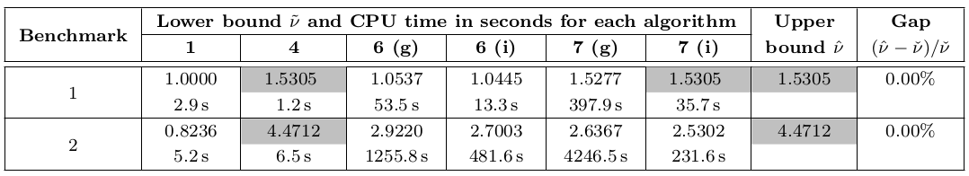
Once again, the most relevant algorithm is the poles migration technique of [1], with both the highest accuracy and the lowest computational time. Indeed, the exact value of $\nu$ is obtained in both cases in only 3.8s on average. The nonsmooth optimization technique of [32] produces mixed results, since the exact value of $\nu$ is obtained for the first benchmark only. Note that much better results are reported in [32] for the second benchmark. Nevertheless, this requires to consider a much larger number of frequency points or intervals, and the computational burden significantly increases. As expected, the power algorithm of [63] fails to converge for a large number of frequencies and returns poor results.
Conclusion
This page provides a thorough comparative analysis of all practical methods to compute lower bounds on the structured singular value $\mu$. The most relevant algorithms are the poles migration technique of [1] for purely real problems and the power algorithm of [2] for purely complex and mixed real/complex problems. Based on these conclusions, simple improvements and combinations are proposed to approach the exact value of $\mu$ with a reasonable computational effort, resulting in state-of-the-art tools. Their evaluation on a wide set of 36 real-world benchmarks available in the litterature shows that non-conservative values can be obtained in almost all cases. Moreover, their extension to handle skew-$\mu$ problems also proves conclusive. All these tools are implemented in the Skew Mu Analysis based Robustness Tools (SMART) library of the SMAC toolbox.
References
| [1] | G. Ferreres and J-M. Biannic, "Reliable computation of the robustness margin for a flexible aircraft", Control Engineering Practice, vol. 9, no. 12, pp. 1267-1278, 2001. |
| [2] | P. Young and J. Doyle, "A lower bound for the mixed $\mu$ problem", IEEE Transactions on Automatic Control, vol. 42, no. 1, pp. 123-128, 1997. |
| [3] | R. De Gaston and M. Safonov, "Exact calculation of the multiloop stability margin", IEEE Transactions on Automatic Control, vol. 33, no. 2, pp. 156-171, 1988. |
| [4] | A. Sideris and R. De Gaston, "Multivariable stability margin calculation with uncertain correlated parameters", in Proceedings of the 25th IEEE Conference on Decision and Control, Athens, Greece, 1986, pp. 766–771. |
| [5] | A. Sideris and R. Sanchez Pena, "Fast computation of the multivariable stability margin for real interrelated uncertain parameters", IEEE Transactions on Automatic Control, vol. 34, no. 12, pp. 1272-1276, 1989. |
| [6] | A. Sideris and R. Sanchez Pena, "Robustness margin calculation with dynamic and real parametric uncertainty", IEEE Transactions on Automatic Control, vol. 35, no. 8, pp. 970-974, 1990. |
| [7] | L. Zadeh and C. Desoer, "Linear system theory", New York: McGraw Hill, 1963. |
| [8] | B. Barmish and H. Kang, "A survey of extreme point results for robustness of control systems", Automatica, vol. 29, no. 1, pp. 13-35, 1993. |
| [9] | A. Bartlett, C. Hollot and H. Lin, "Root locations on an entire polytope of polynomials: it suffices to check the edges", Mathematics of Control, Signals and Systems, vol. 1, no. 1, pp. 61-71, 1988. |
| [10] | R. Dailey, "A new algorithm for the real structured singular value", in Proceedings of the American Control Conference, San Diego, California, 1990, pp. 3036-3040. |
| [11] | M. Elgersma, J. Freudenberg and B. Morton, "Polynomial methods for the structured singular value with real parameters", International Journal of Robust and Nonlinear Control, vol. 6, no. 2, pp. 147-170, 1996. |
| [12] | B. van der Waerden, "Algebra", Springer Verlag, New York, 1991. |
| [13] | T. Matsuda, M. Kawanishi and T. Narikiyo, "Computation of real structured singular value by stability feeler", in Proceedings of the Asian Control Conference, Hong Kong, China, 2009, pp. 672-677. |
| [14] | T. Matsuda and T. Mori, "Stability feeler: a tool for parametric robust stability analysis and its applications", IET Control Theory & Applications, vol. 3, no. 12, pp. 1625-1633, 2009. |
| [15] | P. Young, M. Newlin and J. Doyle, "Computing bounds for the mixed $\mu$ problem", International Journal of Robust and Nonlinear Control, vol. 5, no. 6, pp. 573-590, 1995. |
| [16] | J. Tierno and P. Young, "An improved $\mu$ lower bound via adaptive power iteration", in Proceedings of the 31st IEEE Conference on Decision and Control, Tucson, Arizona, 1992, pp. 3181-3186. |
| [17] | Y. Cheng and B. De Moor, "Continuous power iteration for computing lower bound of $\mu$", in Proceedings of the American Control Conference, Baltimore, Maryland, 1994, pp. 1416-1417. |
| [18] | M. Newlin and S. Glavaski, "Advances in the computation of the $\mu$ lower bound", in Proceedings of the American Control Conference, Seattle, Washington, 1995, pp. 442-446. |
| [19] | J. Dehaene, C. Yi and B. De Moor, "Calculation of the structured singular value with gradient-based optimization algorithms on a Lie group of structured unitary matrices", IEEE Transactions on Automatic Control, vol. 42, no. 11, pp. 1596-1600, 1997. |
| [20] | P. Seiler, A. Packard and G. Balas, "A gain-based lower bound algorithm for real and mixed $\mu$ problems", Automatica, vol. 46, no. 3, pp. 493-500, 2010. |
| [21] | A. Packard, G. Balas, R. Liu and J. Shin, "Results on worst-case performance assessment", in Proceedings of the American Control Conference, Chicago, Illinois, 2000, pp. 2425-2427. |
| [22] | J. Magni, C. Döll, C. Chiappa, B. Frappard and B. Girouart, "Mixed $\mu$-analysis for flexible systems. Part 1: theory", in Proceedings of the 14th IFAC World Congress, Beijing, China, 1999, pp. 325-360. |
| [23] | A. Packard and P. Pandey, "Continuity properties of the real/complex structured singular value", IEEE Transactions on Automatic Control, vol. 38, no. 3, pp. 415-428, 1993. |
| [24] | P. Iordanov and M. Halton, "Computation of the real structured singular value via pole migration", International Journal of Robust and Nonlinear Control, DOI: 10.1002/rnc.3259, 2014. |
| [25] | P. Iordanov, M. Hayes and M. Halton, "On $\mu$-analysis and synthesis for systems subject to real uncertainty", in Proceedings of the 7th European Control Conference, Cambridge, United Kingdom, 2003, pp. 420-425. |
| [26] | M. Hayes, D. Bates and I. Postlethwaite, "New tools for computing tight bounds on the real structured singular value", Journal of Guidance, Control, and Dynamics, vol. 24, no. 6, pp. 1204-1213, 2001. |
| [27] | D. Bates and T. Mannchen, "Improved computation of mixed $\mu$ bounds for flight control law robustness analysis", in Proceedings of the Institution of Mechanical Engineers, Part I: Journal of Systems and Control Engineering, vol. 218, no. 8, pp. 609-619, 2004. |
| [28] | M. Halton, M. Hayes and P. Iordanov, "State-space $\mu$ analysis for an experimental drive-by-wire vehicle", International Journal of Robust and Nonlinear control, vol. 18, pp. 975-992, 2008. |
| [29] | A. Yazıcı, A. Karamancıoglu and R. Kasimbeyli, "A nonlinear programming technique to compute a tight lower bound for the real structured singular value", Optimization and Engineering, vol. 12, no. 3, pp. 445-458, 2011. |
| [30] | R. Kasimbeyli, O. Ustun and A. Rubinov, "The modified subgradient algorithm based on feasible values", Optimization, vol. 58, no. 5, pp. 535-560, 2009. |
| [31] | A. Brito and J. Kim, "Application of a two-step calculation of the real structured singular value to the science mode of the LISA mission", in Proceedings of the AIAA Guidance, Navigation, and Control Conference, Toronto, Canada, 2010. |
| [32] | R. Lemos, A. Simoes and P. Apkarian, "A non-smooth lower bound on $\nu$", International Journal of Robust and Nonlinear Control, vol. 24, no. 3, pp. 477-494, 2014. |
| [33] | J. Kim, D. Bates and I. Postlethwaite, "A geometrical formulation of the $\mu$-lower bound problem", IET Control Theory & Applications, vol. 3, no. 4, pp. 465-472, 2009. |
| [34] | G. Ferreres, J-F. Magni and J-M. Biannic, "Robustness analysis of flexible structures: practical algorithms", International Journal of Robust and Nonlinear Control, vol. 13, pp. 715-734, 2003. |
| [35] | J-M. Biannic and G. Ferreres, "Efficient computation of a guaranteed robustness margin", in Proceedings of the 16th IFAC World Congress, Prague, Czech Republic, 2005. |
| [36] | C. Roos and J-M. Biannic, "Efficient computation of a guaranteed stability domain for a high-order parameter dependent plant", in Proceedings of the American Control Conference, Baltimore, Maryland, 2010, pp. 3895-3900. |
| [37] | C. Lawrence, A. Tits and P. Van Dooren, "A fast algorithm for the computation of an upper bound on the $\mu$-norm", Automatica, vol. 36, no. 3, pp. 449-456, 2000. |
| [38] | A. Sideris, "Elimination of frequency search from robustness tests", IEEE Transactions on Automatic Control, vol. 37, no. 10, pp. 1635-1640, 1992. |
| [39] | M. Fu and N. Barabanov, "Improved upper bounds for the mixed structured singular value", IEEE Transactions on Automatic Control, vol. 42, no. 10, pp. 1447-1452, 1997. |
| [40] | J. Ly, R. Chiang, K. Goh and M. Safonov, "LMI multiplier $K_m/\mu$ analysis of the Cassini spacecraft", International Journal of Robust and Nonlinear Control, vol. 8, no. 2, pp. 155-168, 1998. |
| [41] | J. Lee and T. Edgar, "Upper bounds of structured singular values for mixed uncertainties", in Proceedings of the 42nd IEEE Conference on Decision and Control, Maui, Hawaii, 2003, pp. 798-802. |
| [42] | G. Ferreres, J-M. Biannic and J-F. Magni, "A skew mu toolbox (SMT) for robustness analysis", in Proceedings of the 13th IEEE International Symposium on Computer Aided Control Systems Design, Taipei, Taiwan, 2004, pp. 309-314. |
| [43] | C. Roos, "Systems Modeling, Analysis and Control (SMAC) Toolbox: an insight into the robustness analysis library,” in Proceedings of the IEEE Multiconference on Systems and Control, Hyderabad, India, 2013, pp. 176–181. |
| [44] | R. Braatz and M. Morari, "$\mu$-sensitivities as an aid for robust identification", in Proceedings of the American Control Conference, Boston, Massachusetts, 1991, pp. 231-236. |
| [45] | M. Newlin and P. Young, "Mixed $\mu$ problems and branch and bound techniques", International Journal of Robust and Nonlinear Control, vol. 7, pp. 145-164, 1997. |
| [46] | G. Balas, Private communication, 2014. |
| [47] | The MathWorks, "Robust Control Toolbox", available at http://www.mathworks.com/help/robust/examples/robustness-of-servo-controller-for-dc-motor.html, 2014. |
| [48] | J. Ackermann and W. Sienel, "Robust control for automatic steering", in Proceedings of the American Control Conference, San Diego, California, 1990, pp. 795-800. |
| [49] | J-M. Biannic and C. Roos, Benchmark developed by ONERA - The French Aerospace Lab in cooperation with industrial partners, 2013. |
| [50] | K. Wise, "Comparison of six robustness tests evaluating missile autopilot robustness to uncertain aerodynamics", AIAA Journal of Guidance, Control and Dynamics, vol. 15, no. 4, pp. 861-870, 1992. |
| [51] | P. Seiler, G. Balas and A. Packard, "A gain-based lower bound algorithm for real and mixed $\mu$ problems", in Proceedings of the 45th IEEE Conference on Decision and Control, San Diego, California, 2006, pp. 3548-3553. |
| [52] | R. Vadigepalli, E. Gatzke and F. Doyle III, "Robust control of a multivariable experimental four-tank system", Industrial & Engineering Chemistry Research, vol. 40, no. 8, pp. 1916-1927, 2001. |
| [53] | S. Juliana, "Re-entry flight clearance", Ph.D. dissertation, Delft University of Technology, 2006. |
| [54] | G. Ferreres, "A practical approach to robustness analysis with aeronautical applications", Kluwer Academic, 1999. |
| [55] | J. Ackermann and W. Sienel, "What is a large number of parameters in robust systems?", in Proceedings of the 29th IEEE Conference on Decision and Control, Honolulu, Haiwaii, 1990, pp. 3496-3497. |
| [56] | N. Safari-Shad and M. Takabe, "Refined robust stability analysis of a spark ignition engine model", IEEE Transactions on Control Systems Technology, vol. 5, no. 2, pp. 261-265, 1997. |
| [57] | Y. Cheng and B. De Moor, "Robustness analysis and control system design for a hydraulic servo system", IEEE Transactions on Control System Technology, vol. 2, no. 3, pp. 183-197, 1994. |
| [58] | Z. Ge and L. Chu, "An interval method for computing the stability margin of real uncertainty problems", Optimal Control Applications and Methods, vol. 21, pp. 185-193, 2000. |
| [59] | G. Balas, J. Doyle, K. Glover, A. Packard and R. Smith, "Mu-analysis and synthesis toolbox for use with Matlab", User’s guide, version 3, 2001. |
| [60] | D. Gu, P. Petkov and M. Konstantinov, "Robust control design with Matlab", Advanced Textbooks in Control and Signal Processing, Springer-Verlag, London, 2005. |
| [61] | L. Sanches, D. Alazard, G. Michon and A. Berlioz, "Robustness analysis of helicopter ground resonance with parametric uncertainties in blade properties", AIAA Journal of Guidance, Control and Dynamics, vol. 36, no. 1, pp. 272-281, 2013. |
| [62] | C. Roos, F. Lescher, J-M. Biannic, C. Döll and G. Ferreres, "A set of $\mu$-analysis based tools to evaluate the robustness properties of high-dimensional uncertain systems", in Proceedings of the IEEE Multiconference on Systems and Control, Denver, Colorado, 2011, pp. 644-649. |
| [63] | G. Ferreres and V. Fromion, "Robustness analysis using the $\nu$ tool", in Proceedings of the 35th IEEE Conference on Decision and Control, Kobe, Japan, 1996, pp. 4566-4571. |
| [64] | S. Glavaski and J. Tierno, "Advances in worst-case $H_\infty$ performance computation", in Proceedings of the IEEE Conference on Control Applications, Trieste, Italy, 1998, pp. 668-673. |
| [65] | R. Holland, P. Young and C. Zhu, "Development of a skew $\mu$ lower bound", International Journal of Robust and Nonlinear Control, vol. 15, no. 11, pp. 495-506, 2005. |