Routine mulb_mixed

Compute (skew-)$\mu$ lower bounds for mixed perturbations.

Description

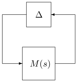
This routine computes (skew-)$\mu$ lower bounds for an interconnection between a nominal LTI system $M(s)$ and a block-diagonal operator $\Delta(s)=diag\left(\Delta_1(s),\dots,\Delta_N(s)\right)$, where $\Delta_i(s)=\delta_iI_{n_i}$ ($\delta_i$ real or complex), or $\Delta_i(s)$ is a stable and proper real-rational unstructured transfer function. A power algorithm is run at each point of a frequency grid. The considered stability region can be bounded either by the imaginary axis or by a truncated sector.

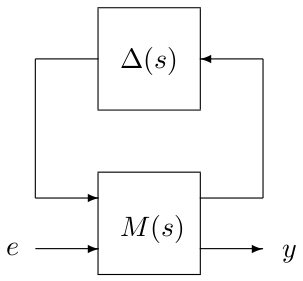
This routine can also be used to solve a worst-case $\mathcal{H}_\infty$ performance problem, which is nothing but a specific skew-$\mu$ problem. A fictitious stable and proper real-rational unstructured transfer matrix $\Delta_c(s)$ is first added between the output $y$ and the input $e$, and its size is then minimized under the constraint that there exists a value of $\Delta(s)\in\mathcal{B}_{\bf\Delta}$ such that the interconnection between $M(s)$ and $diag(\Delta(s),\Delta_c(s))$ is unstable. An example is given at the bottom of this page. In this case, the output argument lbnd is a lower bound on the worst-case $\mathcal{H}_\infty$ norm of the transfer matrix from $e$ to $y$.

Syntax

[lbnd,wc,pert,tab]=mulb_mixed(sys,blk{,options})

Input arguments

The first two input arguments are mandatory:

sys LTI object describing the nominal system $M(s)$. It can also be a 2-D or 3-D numeric array corresponding to the frequency response of $M(s)$ on a grid.

blk

Matrix defining the structure of the block-diagonal operator $\Delta(s)=diag\left(\Delta_1(s),...,\Delta_N(s)\right)$. Its first 2 columns must be defined as follows for all $i=1,...,N$:

blk(i,1:2)=[-ni 0] $\Rightarrow$ $\Delta_i(s)=\delta_iI_{n_i}$ with $\delta_i$ real.
blk(i,1:2)=[ni 0] $\Rightarrow$ $\Delta_i(s)=\delta_iI_{n_i}$ with $\delta_i$ complex,
blk(i,1:2)=[ni ni] $\Rightarrow$ $\Delta_i(s)$ is a $n_i\times n_i$ LTI system.

A third column can be used to specify skew uncertainties:

blk(i,3)=0 $\Rightarrow$ $\overline{\sigma}(\Delta_i(j\omega))\le 1$ for all $\omega\in\Omega$,
blk(i,3)=1 $\Rightarrow$ $\overline{\sigma}(\Delta_i(j\omega))\le 1/$lbnd for all $\omega\in\Omega$, where lbnd is maximized.

If none, blk(i,3) is set to 1 for all $i=1,...,N$.

The third input argument options is an optional structured variable with fields:

`freq`	Frequency interval $\Omega$ in rad/s on which the lower bound is to be computed. The default value is `options.freq=[0 10*max(abs(eig(sys)))]`. This parameter is ignored if `sys` is a numeric array.
`grid`	Frequency grid in rad/s ($1\times m$ array). It can also be a negative integer -$m$, in which case a $m$-point grid is automatically generated from $\Omega$. The default value is `options.grid=-50`. This parameter is ignored if `sys` is a numeric array.
`sector`	Vector $[\alpha\ \xi]$ or $[\alpha\ \xi\ \omega_c]$ characterizing the considered truncated sector (see `display_sector` for a complete description). The default value is `options.sector=[0 0]`, which means that the left half plane is considered. This parameter is ignored if `sys` is a numeric array.
`target`	The algorithm is interrupted if a lower bound is found which is greater than `options.target`. The default value is `options.target=Inf`.
`epsilon`	A (skew-)$\mu$ lower bound $\tilde{\mu}$ is acceptable if a perturbation $\tilde{\Delta}$ of norm 1/$\tilde{\mu}$ and a frequency $\omega_c$ are found, which satisfy $\|\mbox{det}(I-M(j\omega_c)\tilde{\Delta})\|<\epsilon$, where $M(j\omega_c)$ is the frequency response of $M(s)$ at $j\omega_c$ (or at the corresponding point on the boundary of the truncated sector defined by `options.sector`). The default value is `options.epsilon=1e-8`.
`trace`	Trace of execution. The default value is `options.trace=1`.
`warn`	Warnings display. The default value is `options.warn=1`.
`power`	Tuning parameters of the power algorithm (1x4 array). At each frequency: a run using the previous results as an initialization is performed if `options.power(1)` is nonzero. a run with a deterministic initialization is performed if `options.power(2)` is nonzero. `options.power(3)` runs are performed with a random initialization. at most `options.power(4)` iterations are performed at each run. The default value is `options.power=[1 0 1 100]`.
`refine`	If nonzero, the initial frequency grid is refined near peak values of the (skew-)$\mu$ lower bound. The default value is `options.refine=1`. This parameter is ignored if `sys` is a numeric array.

Output arguments

`lbnd`	Best (skew-)$\mu$ lower bound on the considered frequency interval $\Omega$.
`wc`	Frequency $\omega_c$ in rad/s for which `lbnd` has been computed.
`pert`	Unless `lbnd=0`, every perturbation $\tilde{\Delta}(s)$ whose frequency response $\tilde{\Delta}(\omega_c)$ at $j\omega_c$ (or at the corresponding point on the boundary of the truncated sector defined by `options.sector`) is equal to `pert` satisfies $\mbox{det}(I-M(\omega_c)\tilde{\Delta}(\omega_c))\approx 0$, where $M(\omega_c)$ is the frequency response of $M(s)$.
`tab`	Structured variable with fields: `lbnd`: other (skew-)$\mu$ lower bounds ($m\times 1$ array). `wc`: associated frequencies in rad/s ($m\times 1$ array). `pert`: associated destabilizing perturbations ($n\times n\times m$ array, where $n=\displaystyle\sum_{i=1}^{N}{n_i}$).

Examples

1. Computation of a skew-$\mu$ lower bound

System with 10 states and 3 uncertainties. The second one is kept inside the unit ball:
sys=rss(10,5,5)/100;
blk=[-2 0 1;-1 0 0;2 2 1];
options.sector=[0.1 0];
[lbnd,wc,pert]=mulb_mixed(sys,blk,options);lbnd display_sector(options.sector,lft(sys,pert));
One of the eigenvalues of the interconnection lies just outside the considered sector.
abs(det(eye(5)-calc_freq_resp(sys,wc,options.sector)*pert))
The value of $\mbox{det}(I-M(\omega_c)\tilde{\Delta}(\omega_c))$ is almost equal to 0.

2. Computation of a lower bound on the worst-case $\mathcal{H}_\infty$ norm

System with 10 states and 2 uncertainties, which are both kept inside the unit ball. The third block of $\Delta(s)$ corresponds to the performance channel:
blk=[-2 0 0;-1 0 0;2 2 1];
[lbnd,wc,tab]=mulb_mixed(sys,blk,options);lbnd

Reference