Routine muub_mixed

Compute (skew-)$\mu$ upper bounds for mixed perturbations.

Description

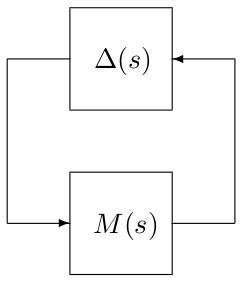
This routine computes a (skew-)$\mu$ upper bound for an interconnection between a nominal LTI system $M(s)$ and a block-diagonal operator $\Delta(s)= diag\left(\Delta_1(s),\dots,\Delta_N(s)\right)$. A bound and associated $D$ and $G$ scaling matrices are first computed at a given frequency. The largest frequency interval on which they remain valid is then obtained. This strategy is repeated until the whole frequency range is covered which leads to a guaranteed upper bound. The considered stability region can be bounded either by the imaginary axis or by a truncated sector.

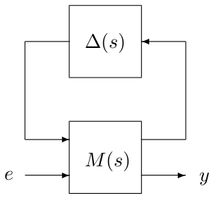
This routine can also be used to solve a worst-case $\mathcal{H}_\infty$ performance problem, which is nothing but a specific skew-$\mu$ problem. A fictitious stable and proper real-rational unstructured transfer matrix is first added between the output $y$ and the input $e$, and its size is then maximized under the constraint that the interconnection is stable $\forall\Delta(s)\in\mathcal{B}_{\bf\Delta}$. An example is given at the bottom of this page. In this case, the output argument ubnd is a guaranteed upper bound on the worst-case $\mathcal{H}_\infty$ norm of the transfer matrix from $e$ to $y$.

Syntax

[ubnd,wc,tab,pb]=muub_mixed(sys,blk{,options})

Input arguments

The first two input arguments are mandatory:

sys

LTI object describing the nominal system $M(s)$.

blk

Matrix defining the structure of the block-diagonal operator $\Delta(s)=diag\left(\Delta_1(s),...,\Delta_N(s)\right)$. Its first 2 columns must be defined as follows for all $i=1,...,N$:

blk(i,1:2)=[-ni 0] $\Rightarrow$ $\Delta_i(s)=\delta_iI_{n_i}$ with $\delta_i$ real,
blk(i,1:2)=[ni 0] $\Rightarrow$ $\Delta_i(s)=\delta_iI_{n_i}$ with $\delta_i$ complex,
blk(i,1:2)=[ni ni] $\Rightarrow$ $\Delta_i(s)$ is a $n_i\times n_i$ LTI system.

A third column can be used to specify skew uncertainties:

blk(i,3)=0 $\Rightarrow$ $\overline{\sigma}(\Delta_i(j\omega))\le 1$ for all $\omega\in\Omega$,
blk(i,3)=1 $\Rightarrow$ $\overline{\sigma}(\Delta_i(j\omega))\le 1/$ubnd for all $\omega\in\Omega$, where ubnd is minimized.

If none, blk(i,3) is set to 1 for all $i=1,...,N$.

The third input argument options is an optional structured variable with fields:

w0	Starting frequency point in rad/s. The default value is options.w0=0.
freq	Frequency interval $\Omega$ in rad/s on which the upper bound is to be computed. The default value is options.freq=[0 max([10*abs(eig(sys)) options.w0])]).
sector	Vector $[\alpha\ \xi]$ or $[\alpha\ \xi\ \omega_c]$ characterizing the considered truncated sector (see display_sector for a complete description). The default value is options.sector=[0 0], which means that the left half plane is considered.
lmi	If options.lmi=1, the LMI-based characterization of a (skew-)$\mu$ upper bound is used instead of the $\overline{\sigma}$-based one for better accuracy. The default value is options.lmi=0. Note that setting options.lmi=1 in the presence of highly repeated parametric uncertainties (i.e. blocks $\Delta_i(s)=\delta_iI_{n_i}$ with $n_i\ge 10$), may lead to high computational costs.
trace	Trace of execution. The default value is options.trace=1.
warn	Warnings display. The default value is options.warn=1.
target	Value of the upper bound above which the algorithm is interrupted. The default value is options.target=Inf.
init	Initial guess (typically a (skew)-$\mu$ lower bound). The default value is options.init=0.
reg	Regularization for real-$\mu$ problems. The default value is options.reg=0.01, i.e. 1% of complex uncertainty is added in case of convergence problems.
tol	At each iteration, the (skew-)$\mu$ upper bound is increased by a factor of 1+options.tol before the interval on which the scaling matrices are valid is computed. The default value is options.tol=0.01.
maxiter	Maximum number of iterations. The default value is options.maxiter=1000.
elim	A pawl effect on $\mu$ is used to fasten the elimination technique if options.elim=1. Better estimates of secondary peaks are obtained if options.elim=0. The default value is options.elim=1.
smm	Method for the iterative calls to mussv in case of a skew-$\mu$ problem (1 $\Leftrightarrow$ fixed-point algorithm, 2 $\Leftrightarrow$ dichotomy search). The default value is options.smm=1. This option is ignored if options.lmi is nonzero.

Output arguments

ubnd	(Skew-)$\mu$ upper bound on the considered frequency interval $\Omega$.
wc	Frequency in rad/s for which ubnd has been computed.
tab	Structured variable with fields (see plot_muub): ubnd: (skew-)$\mu$ upper bounds. int: frequency intervals on which the upper bounds are valid.
pb	Indicates a convergence problem when non-zero: 1 $\Rightarrow$ impossible to further eliminate intervals. 2 $\Rightarrow$ maximum number of iterations reached. 3 $\Rightarrow$ skew-$\mu$ problem infeasible. 4 $\Rightarrow$ $\mu$-test failed.

Examples

1. Computation of a $\mu$ upper bound

System with 46 states and 20 non-repeated real parametric uncertainties:

load flexible_airplane 
[ubnd,wc,tab]=muub_mixed(sys,blk);ubnd 
Improvement of the result at the price of a higher computational time: 
options.tol=0; 
options.lmi=1; 
[ubnd,wc,tab]=muub_mixed(sys,blk,options);ubnd 
Computation on a limited frequency range: 
options.freq=[0 10]; 
[ubnd,wc,tab]=muub_mixed(sys,blk,options);ubnd

2. Computation of a skew-$\mu$ upper bound

System with 10 states and 3 uncertainties. The second one is kept inside the unit ball:

sys=rss(10,5,5);
sys=ss(sys.a-0.1*eye(10),sys.b/10,sys.c/10,sys.d/100);
blk=[-2 0 1;-1 0 0;2 2 1]; [ubnd,wc,tab]=muub_mixed(sys,blk);ubnd

3. Computation of an upper bound on the worst-case $\mathcal{H}_\infty$ norm

System with 10 states and 2 uncertainties, which are both kept inside the unit ball. The third block of $\Delta(s)$ corresponds to the performance channel:

blk=[-2 0 0;-1 0 0;2 2 1];
[ubnd,wc,tab]=muub_mixed(sys,blk);ubnd

References