Routine hinflb_real

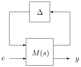
Compute lower bounds on the worst-case $\mathcal{H}_\infty$ norm for real perturbations.

Description

This routine computes lower bounds on the worst-case $\mathcal{H}_\infty$ norm for an interconnection between a nominal LTI system $M(s)$ and a block-diagonal operator $\Delta=diag\left(\Delta_1,\dots,\Delta_N\right)$, where $\Delta_i=\delta_iI_{n_i}$ and $\delta_i$ is real. Lower bounds are first computed on a rough frequency grid. A series of quadratic programming problems is then solved using these results as an initialization.

Let $\mathcal{B}_{\bf\Delta}$ be the set of all admissible block-diagonal operators $\Delta$ such that $|\delta_i|<1$ for all $i=1,\dots,N$. Assume that the interconnection between $M(s)$ and $\Delta$ is stable for all $\Delta\in\mathcal{B}_{\bf\Delta}$. Let $\mathcal{F}_u(M(s),\Delta)$ denote the transfer matrix from $e$ to $y$, which must be square (see make_square). The worst-case $\mathcal{H}_\infty$ norm is defined by:
$$\max_{\Delta\in\mathcal{B}_{\bf\Delta}} \|\mathcal{F}_u(M(s),\Delta)\|_\infty$$
where the $\mathcal{H}_\infty$ norm can be computed either on the imaginary axis or on the boundary of a truncated sector.

Note: The aim is not to compute a lower bound as a function of frequency but to compute a lower bound over the whole frequency range. The frequency for which the largest singular value of the transfer matrix from $e$ to $y$ is maximum is left free during the optimization and can be very far from the initial one. Thus, a rough initial grid is usually sufficient to capture the most critical frequencies.

Syntax

[lbnd,wc,pert,tab]=hinflb_real(sys,blk{,options})

Input arguments

The first two input arguments are mandatory:

sys LTI object describing the nominal system $M(s)$.

blk

Matrix defining the structure of the block-diagonal operator $\Delta=diag\left(\Delta_1,...,\Delta_N\right)$. Its first 2 columns must be defined as follows for all $i=1,...,N$:

blk(i,1:2)=[-ni 0] $\Rightarrow$ $\Delta_i=\delta_iI_{n_i}$ with $\delta_i$ real.

The third input argument options is an optional structured variable with fields:

freq	Frequency interval $\Omega$ in rad/s on which the lower bound is to be computed. The default value is `options.freq=[0 10*max(abs(eig(sys)))]`.
grid	Frequency grid in rad/s ($1\times m$ array). It can also be a negative integer -$m$, in which case a $m$-point grid is automatically generated from $\Omega$. The default value is `options.grid=-10`.
sector	Vector $[\alpha\ \xi]$ or $[\alpha\ \xi\ \omega_c]$ characterizing the considered truncated sector (see display_sector for a complete description). The default value is options.sector=[0 0], which means that the left half plane is considered.
target	The algorithm is interrupted if a lower bound is found which is greater than options.target. The default value is options.target=Inf.
trace	Trace of execution. The default value is `options.trace=1`.
warn	Warnings display. The default value is `options.warn=1`.
wpar	If zero, frequency is treated as an additional parameter in $\Delta$ and the problem is solved on the intervals `[grid(1) grid(2)],...,[grid(end-1) grid(end)]`. The default value is `options.wpar=0`.
prec	Level of precision of the final result (`options.prec=2` $\Leftrightarrow$ good precision, `options.prec=1` $\Leftrightarrow$ faster but potentially less precise). The default value is `options.prec=1`.
local	If zero, the algorithm focuses on the global worst-case configuration. Otherwise, it also tries to detect local maxima, but the probability to determine the global worst-case configuration is lower. The default value is `options.local=0`.
method	$1\times 2$ array defining the method used for the line search: `options.method=[1 tol]` means that the optimum is computed from the real eigenvalues of a hamiltonian matrix with a precision of `tol`. `options.method=[2 m]` means that the optimum is computed on a grid composed of $m$ points. `options.method=[1 tol]` is often more accurate but CPU time is higher. The default value is `options.method=[1 0.001]` or `[2 6]` depending on the size of $\Delta$ (less or more than 50).

Output arguments

lbnd	Best lower bound on the worst-case $\mathcal{H}_\infty$ norm on the considered frequency interval $\Omega$.
wc	Frequency $\omega_c$ in rad/s for which `lbnd` has been computed.
pert	Associated value of $\tilde{\Delta}$: unless `lbnd=0`, the largest singular value of $\mathcal{F}_u(M(\omega_c),\tilde{\Delta})$ is equal to `lbnd`, where $M(\omega_c)$ is the frequency response of $M(s)$ at $j\omega_c$ (or at the corresponding point on the boundary of the truncated sector defined by `options.sector`).
tab	Structured variable with fields: `lbnd`: other lower bounds on the worst-case $\mathcal{H}_\infty$ norm ($m\times 1$ array). `wc`: associated frequencies in rad/s ($m\times 1$ array). `pert`: associated values of $\tilde{\Delta}$ ($n\times n\times m$ array, where $n=\displaystyle\sum_{i=1}^{N}{n_i}$).

Example

System with 10 states and 2 uncertainties. The last two inputs and outputs correspond to the performance channel:
sys=rss(10,5,5);
sys=ss(sys.a-0.1*eye(10),sys.b/10,sys.c/10,sys.d/100);
blk=[-2 0;-1 0];
options.sector=[-0.05 0]; [lbnd,wc,pert,tab]=hinflb_real(sys,blk,options); max(svd(lft(pert,calc_freq_resp(sys,wc,options.sector))))-lbnd

Reference