Compute bounds on the worst-case gain, phase, modulus and delay margins with desired accuracy.
Description
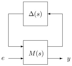
Let us consider the following interconnection between a nominal LTI system $M(s)$ and a block-diagonal operator $\Delta(s)$.
Lower and/or upper bounds $M_{lb}$ and $M_{ub}$ are computed on the highest value $M_{max}$ of the (real or complex) gain, the phase shift or the time-delay that can be inserted between $y$ and $e$ without destabilizing the interconnection when $\Delta(s)$ takes any admissible value (see problem 3 on the overview page of the toolbox or more details). More precisely, some additional fictitious uncertainties $\delta_{M}=diag(\delta_{M,i})$ corresponding to gain, phase, modulus or time-delay variations are connected between $y$ and $e$ (see also the example at the bottom of this page):
- $\delta_{M,i}=1+\hat{\delta}_i$, where $\hat{\delta}_i$ is real, if the worst-case gain margin is to be evaluated,
- $\delta_{M,i}=e^{j\hat{\delta}_i}$, where $\hat{\delta}_i$ is real, if the worst-case phase margin is to be evaluated,
- $\delta_{M,i}=1+\hat{\delta}_i$, where $\hat{\delta}_i$ is complex, if the worst-case modulus margin is to be evaluated,
- $\delta_{M,i}=e^{-\hat{\delta}_is}$, where $\hat{\delta}_i$ is positive real, if the worst-case delay margin is to be evaluated.
In this context, the value of $M_{max}$ corresponds to the maximum value of $|\hat{\delta_i}|$ for which the interconnection is stable for any admissible value of $\Delta(s)$. The lower bound $M_{lb}$ is guaranteed on a whole frequency interval. Moreover, a branch and bound algorithm can be applied, in which case the bounds satisfy $M_{ub}\le (1+\epsilon)M_{lb}$, where $\epsilon$ is a user-defined threshold. A value $\tilde{\Delta}(s)$ of $\Delta(s)$ for which the upper bound $M_{ub}$ is obtained is also determined, and the considered stability region can be bounded either by the imaginary axis or by a truncated sector. Note: The initial interconnection is normalized with convert_data before the problem is solved.
Syntax
[bnds,wc,pert,iodesc]=iomargins(usys,margin{,options}) [bnds,wc,pert,iodesc]=iomargins(gsys,margin{,options}) [bnds,wc,pert,iodesc]=iomargins(lsys,margin{,options}) [bnds,wc,pert,iodesc]=iomargins(sys,blk,margin{,options})
Input arguments
The interconnection between $M(s)$ and $\Delta(s)$ can be described by:
- a USS object
usys, - a GSS object
gsys, - a LFR object
lsys, - a LTI object
sysdescribing the LTI system $M(s)$ and a $N\times 2$ matrixblkdefining the structure of the block-diagonal operator $\Delta(s)=diag\left(\Delta_1(s),\dots,\Delta_N(s)\right)$:blk(i,:)=[-ni 0]$\Rightarrow$ $\Delta_i(s)=\delta_iI_{n_i}$ with $\delta_i$ real,blk(i,:)=[ni 0]$\Rightarrow$ $\Delta_i(s)=\delta_iI_{n_i}$ with $\delta_i$ complex,blk(i,:)=[ni mi]$\Rightarrow$ $\Delta_i(s)$ is a $n_i\times m_i$ LTI system.
The second input argument margin is a character array which allows to specify the considered problem:
- it must contain exactly one of the following characters :
'g'for gain margin,'p'for phase margin,'m'for modulus margin or'd'for delay margin, - it must also contain
'l','u','lu'or'b'depending on whether only a lower bound, only an upper bound, both lower and upper bounds, or both lower and upper bounds with desired accuracy have to be computed.
The last input argument options is an optional structured variable with fields:
| freq | Frequency interval $\Omega$ in rad/s on which the bounds are to be computed. The default value is options.freq=[0 10*max(abs(eig(sys)))].Frequency interval Ω in rad/s on which the bounds are to be computed. The default value is options.freq=[0 10*max(abs(eig(sys)))]. |
| sector | Vector $[\alpha\ \xi]$ or $[\alpha\ \xi\ \omega_c]$ characterizing the considered truncated sector (see display_sector for a complete description). The default value is options.sector=[0 0], which means that the left half plane is considered. |
| target | The algorithm is interrupted if the lower or the upper bound on the considered margin becomes lower than options.target. This parameter is ignored if branch and bound is requested, i.e. if margin contains the character 'b'. The default value is options.target=0. |
| lmi | If options.lmi=1, the LMI-based characterization of a (skew-)$\mu$ upper bound is used instead of the $\overline{\sigma}$-based one for better accuracy. This parameter is ignored if only $M_{ub}$ has to be computed, i.e. if margin does not contains the character 'l' or 'b'. The default value is options.lmi=0. Note that setting options.lmi=1 in the presence of highly repeated parametric uncertainties (i.e. blocks $\Delta_i(s)=\delta_iI_{n_i}$ with $n_i\ge 10$), may lead to high computational costs. |
| maxgap | Maximum gap between the bounds. This parameter is considered only if branch and bound is requested, i.e. if margin contains the character 'b'. The default value is options.maxgap=0.05, i.e. 5%. |
| trace | Trace of execution. The default value is options.trace=1. |
| warn | Warnings display. The default value is options.warn=1. |
Additional fields can be defined (see muub_mixed for lower bound computation, mulb_mixed or mulb_nreal for upper bound computation and mubb_mixed for branch and bound), but the ones listed above are usually sufficient for non-expert users.
Output arguments
| bnds | Lower and upper bounds $M_{lb}$ and $M_{ub}$ on the worst-case gain, phase, modulus or delay margin on the considered frequency interval $\Omega$. |
| wc | Frequency $\omega_c$ in rad/s for which $M_{ub}$ has been computed. |
| pert | The gain, phase, modulus or delay margin of the normalized interconnection is less than or equal to $M_{ub}$ for every perturbation $\tilde{\Delta}(s)$ whose frequency response $\tilde{\Delta}(p(\omega_c))$ is equal to pert, where $p(\omega_c)$ denotes the point $j\omega_c$ on the imaginary axis or the corresponding point on the boundary of the truncated sector defined by options.sector. |
| iodesc | Cell array of structured variables:
The last cell of
|
Example
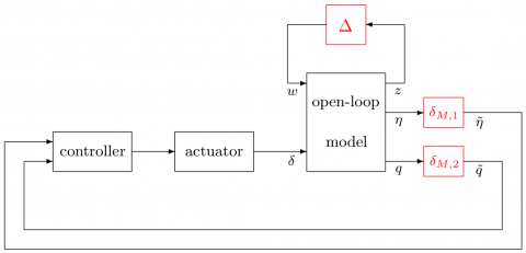
Let us consider the longitudinal missile model depicted in the figure below. The open-loop model has two states (angle of attack and pitch rate), one input (tail fin deflection $\delta$) and two outputs (acceleration $\eta$ and pitch rate $q$). Four parametric uncertainties on the stability derivatives are considered. The open-loop model can thus be written as an LFR, where $\Delta=diag(\delta_1,\delta_2,\delta_3,\delta_4)$. Each of the $\delta_i$ is normalized and the corresponding stability derivative varies by $\pm 50\%$ when $\delta_i\in [-1,1]$. The actuator is modeled by a second order system with frequency $\omega_a=$150 rad/s and damping ratio $\xi_a=$0.7. The controller has 10 states and is designed by an $\mathcal{H}_\infty$ method. Thus the whole plant has 14 states and 4 non-repeated parametric uncertainties.
The objective is to compute reliable estimates of the worst-case gain, phase, modulus and delay margins at the output of the plant when $\Delta$ takes all possible values in the unit ball of admissible perturbations. Two additional inputs $\tilde{\eta},\tilde{q}$ and outputs $\eta,q$ are thus created, and the missile model sys to be used with iomargins is depicted in black in the figure above.load missile_modelminfo(sys)blk=[-1 0;-1 0;-1 0;-1 0]
The first 4 inputs $w$ and outputs $z$ of sys correspond to the parametric uncertainties $\delta_1$ to $\delta_4$, while the last 2 inputs $\tilde{\eta},\tilde{q}$ and outputs $\eta,q$ are used for worst-case margins computation. Note that the $\delta_{M,i}$ are not included in blk.
Optional arguments for lower bound computation:options.lmi=[0.001 100 1e10 5 1];options.tol=0;
1. Worst-case gain margin
Let $\delta_{M,i}=1+\hat{\delta}_i$, where $\hat{\delta}_i$ is real. The worst-case gain margin is the highest value of $M$ such that the interconnection is stable for all $\Delta\in\mathcal{B}_{{\bf\Delta}}$ and for all $|\hat{\delta}_i| < M$.
Computation of lower and upper bounds:[bnds,wc,pert,iodesc]=iomargins(sys,blk,'glu',options);(bnds(2)-bnds(1))/bnds(1)
The gap between the bounds is 0.01%.D=mdiag(pert,eye(2)+diag(iodesc{5}.value));damp(feedback(sys,D,1))
Two eigenvalues of the interconnection lie on the imaginary axis.
2. Worst-case phase margin
Let $\delta_{M,i}=e^{j\hat{\delta}_i}$, where $\hat{\delta}_i$ is real. The worst-case gain margin is the highest value of $M$ such that the interconnection is stable for all $\Delta\in\mathcal{B}_{{\bf\Delta}}$ and for all $|\hat{\delta}_i| < M$.
Computation of lower and upper bounds: bnds,wc,pert,iodesc]=iomargins(sys,blk,'plu',options);(bnds(2)-bnds(1))/bnds(1)
The gap between the bounds is 0.04%.D=mdiag(pert,diag(exp(sqrt(-1)*iodesc{5}.value)));damp(feedback(sys,D,1))
One eigenvalue of the interconnection lies on the imaginary axis.
3. Worst-case modulus margin
Let $\delta_{M,i}=1+\hat{\delta}_i$, where $\hat{\delta}_i$ is complex. The worst-case modulus margin is the highest value of $M$ such that the eigenvalues of the interconnection are inside the considered sector for all $\Delta\in\mathcal{B}_{{\bf\Delta}}$ and for all $|\hat{\delta}_i| < M$.options.sector=[-0.3 0.2];
Computation of lower and upper bounds:[bnds1,wc,pert,iodesc]=iomargins(sys,blk,'mlu',options);(bnds1(2)-bnds1(1))/bnds1(1)
The gap between the bounds is 0.0002%.D=mdiag(pert,eye(2)+diag(iodesc{5}.value)); display_sector(options.sector,feedback(sys,D,1));
One eigenvalue of the interconnection lies on the boundary of the considered sector. options=rmfield(options,'sector');
4. Worst-case delay margin
Let $\delta_{M,i}=e^{-\hat{\delta}_is}$, where $\hat{\delta}_i$ is positive real. The worst-case delay margin is the highest value of $M$ such that the interconnection is stable for all $\Delta\in\mathcal{B}_{{\bf\Delta}}$ and for all $0\le \hat{\delta}_i < M$.
Computation of lower and upper bounds:options.grid=-20;[bnds1,wc,pert,iodesc]=iomargins(sys,blk,'dlu',options);(bnds1(2)-bnds1(1))/bnds1(1)
The gap between the bounds is 1%.s=tf('s');D=mdiag(pert,exp(-iodesc{5}.value(1)*s),exp(-iodesc{5}.value(2)*s));damp(pade(feedback(sys,D,1),5))
One eigenvalue of the interconnection lies on the imaginary axis.
See also
muub_mixed
mulb_mixed
mulb_nreal
hinflb_real
mubb_mixed
convert_data
make_square
References
| [1] | C. Roos, F. Lescher, J-M. Biannic, C. Doll and G. Ferreres, "A set of $\mu$-analysis based tools to evaluate the robustness properties of high-dimensional uncertain systems", in Proceedings of the IEEE Multiconference on Systems and Control, Denver, Colorado, September 2011, pp. 644-649. |
| [2] | F. Lescher and C. Roos, "Robust stability of time-delay systems with structured uncertainties: a $\mu$-analysis based algorithm", in Proceedings of the 50th IEEE Conference on Decision and Control, Orlando, Florida, December 2011, pp.4955-4960. |


