Compute $\mu$ lower bounds for a single real perturbation.
Description
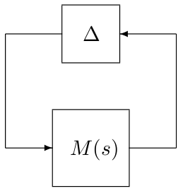
This routine computes $\mu$ lower bounds for an interconnection between a nominal LTI system $M(s)$ and a block-diagonal operator $\Delta=diag\left(\Delta_1,\dots,\Delta_N\right)$, where $\Delta_i=\delta_iI_{n_i}$ and $\delta_i$ is real. Only one uncertainty is allowed to vary at a time. $N$ bounds are thus computed and the ith one corresponds to the inverse of the smallest destabilizing value of $\delta_i$ when $\delta_k=0$ for all $k\ne i$. The considered stability region can be bounded either by the imaginary axis or by a truncated sector.
Note: The aim is not to compute a $\mu$ lower bound as a function of frequency, but to compute a lower bound over the whole frequency range.
Syntax
[lbnd,wc,pert,tab]=mulb_1real(sys,blk{,options})
Input arguments
The first two input arguments are mandatory:
sys | LTI object describing the nominal system $M(s)$. |
blk | Matrix defining the structure of the block-diagonal operator $\Delta=diag\left(\Delta_1,...,\Delta_N\right)$. Its first 2 columns must be defined as follows for all $i=1,...,N$:
|
The third input argument options is an optional structured variable with fields:
freq | Frequency interval $\Omega$ in rad/s on which the lower bound is to be computed. The default value is options.freq=[0 10*max(abs(eig(sys)))]. |
sector | Vector $[\alpha\ \xi]$ or $[\alpha\ \xi\ \omega_c]$ characterizing the considered truncated sector (see display_sector for a complete description). The default value is options.sector=[0 0], which means that the left half plane is considered. |
target | The algorithm is interrupted if a lower bound is found which is greater than options.target. The default value is options.target=Inf. |
epsilon | A $\mu$ lower bound $\tilde{\mu}$ is acceptable if a perturbation $\tilde{\Delta}$ of norm 1/$\tilde{\mu}$ and a frequency $\omega_c$ are found, which satisfy $|\mbox{det}(I-M(j\omega_c)\tilde{\Delta})|<\epsilon$, where $M(j\omega_c)$ is the frequency response of $M(s)$ at $j\omega_c$ (or at the corresponding point on the boundary of the truncated sector defined by options.sector). The default value is options.epsilon=1e-8. |
trace | Trace of execution. The default value is options.trace=1. |
warn | Warnings display. The default value is options.warn=1. |
kmax | Largest considered perturbation. The default value is options.kmax=100. |
npts | Maximum number of equally-spaced values of each $\delta_i$ in [0 options.kmax] for which the stability of the interconnection is checked. The default value is options.npts=1000. |
Output arguments
lbnd | Best $\mu$ lower bound on the considered frequency interval $\Omega$. |
wc | Frequency $\omega_c$ in rad/s for which lbnd has been computed. |
pert | Associated destabilizing perturbation $\tilde{\Delta}$: unless lbnd=0, $\mbox{det}(I-M(\omega_c)\tilde{\Delta})\approx 0$, where $M(\omega_c)$ is the frequency response of $M(s)$ at $j\omega_c$ (or at the corresponding point on the boundary of the truncated sector defined by options.sector). |
tab | Structured variable with fields:
|
Examples
System with 10 states and 1 repeated real parametric uncertainty:sys=rss(10,4,4);blk=[-4 0];options.sector=[0.1 0];[lbnd,wc,pert,tab]=mulb_1real(sys,blk,options);lbnd display_sector(options.sector,lft(sys,pert));check_stab(lft(sys,pert),options.sector)
One of the eigenvalues of the interconnection lies just outside the considered sector.abs(det(eye(4)-calc_freq_resp(sys,wc,options.sector)*pert))
The value of $\mbox{det}(I-M(\omega_c)\tilde{\Delta})$ is almost equal to 0.
System with 46 states and 20 non-repeated real parametric uncertainties:load flexible_airplane options.sector=[-0.05 0.01]; [lbnd,wc,pert,tab]=mulb_1real(sys,blk,options);lbnd display_sector(options.sector,lft(sys,pert));check_stab(lft(sys,pert),options.sector)
One of the eigenvalues of the interconnection lies just outside the considered sector.abs(det(eye(20)-calc_freq_resp(sys,wc,options.sector)*pert))
The value of $\mbox{det}(I-M(\omega_c)\tilde{\Delta})$ is almost equal to 0.