Routine mulb_nreal

Compute (skew-)$\mu$ lower bounds for real perturbations.

Description

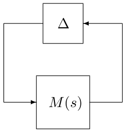
This routine computes (skew-)$\mu$ lower bounds for an interconnection between a nominal LTI system $M(s)$ and a block-diagonal operator $\Delta=diag\left(\Delta_1,\dots,\Delta_N\right)$, where $\Delta_i=\delta_iI_{n_i}$ and $\delta_i$ is real. At each point of a rough frequency grid, a power algorithm is run on a regularized problem and a series of LP problems is solved starting from the real part $\Delta_R$ of the resulting destabilizing perturbation (which usually brings the interconnection close to instability). The considered stability region can be bounded either by the imaginary axis or by a truncated sector.

Note: The aim is not to compute a (skew-)$\mu$ lower bound as a function of frequency, but to compute a lower bound over the whole frequency range. The frequency at which the interconnection becomes unstable is left free during the optimization and can be very far from the initial one. Thus, a rough initial grid is usually sufficient to capture the most critical frequencies.

Syntax

[lbnd,wc,pert,tab]=mulb_nreal(sys,blk{,options})

Input arguments

The first two input arguments are mandatory:

sys LTI object describing the nominal system $M(s)$.

blk

Matrix defining the structure of the block-diagonal operator $\Delta=diag\left(\Delta_1,...,\Delta_N\right)$. Its first 2 columns must be defined as follows for all $i=1,...,N$:

blk(i,1:2)=[-ni 0] $\Rightarrow$ $\Delta_i=\delta_iI_{n_i}$ with $\delta_i$ real.

A third column can be used to specify skew uncertainties:

blk(i,3)=0 $\Rightarrow$ $\overline{\sigma}(\Delta_i)\le 1$,
blk(i,3)=1 $\Rightarrow$ $\overline{\sigma}(\Delta_i)\le 1/$lbnd, where lbnd is maximized.

If none, blk(i,3) is set to 1 for all $i=1,...,N$.

The third input argument options is an optional structured variable with fields:

`freq`	Frequency interval $\Omega$ in rad/s on which the lower bound is to be computed. The default value is `options.freq=[0 10*max(abs(eig(sys)))]`.
`grid`	Frequency grid in rad/s ($1\times m$ array). It can also be a negative integer -$m$, in which case a $m$-point grid is automatically generated from $\Omega$. The default value is `options.grid=-10`.
`sector`	Vector $[\alpha\ \xi]$ or $[\alpha\ \xi\ \omega_c]$ characterizing the considered truncated sector (see `display_sector` for a complete description). The default value is `options.sector=[0 0]`, which means that the left half plane is considered.
`target`	The algorithm is interrupted if a lower bound is found which is greater than `options.target`. The default value is `options.target=Inf`.
`epsilon`	A (skew-)$\mu$ lower bound $\tilde{\mu}$ is acceptable if a perturbation $\tilde{\Delta}$ of norm 1/$\tilde{\mu}$ and a frequency $\omega_c$ are found, which satisfy $\|\mbox{det}(I-M(j\omega_c)\tilde{\Delta})\|<\epsilon$, where $M(j\omega_c)$ is the frequency response of $M(s)$ at $j\omega_c$ (or at the corresponding point on the boundary of the truncated sector defined by `options.sector`). The default value is `options.epsilon=1e-8`.
`trace`	Trace of execution. The default value is `options.trace=1`.
`warn`	Warnings display. The default value is `options.warn=1`.
`method`	Type of LP problem: If `options.method=1`, the scalar $\alpha$ is increased or decreased until the interconnection between $M(s)$ and $\alpha\Delta_R$ is marginally stable. If `options.method=2`, the eigenvalue of the interconnection between $M(s)$ and $\Delta_R$ is identified, which is the closest to the considered point on the boundary of the stability region. When shifting this eigenvalue toward instability, the infinity norm of the model perturbation $\Delta$ is minimized. The default value is `options.method=2`. If this method fails, try to set `options.method=1` instead. Note that the variable `options.method` can also be equal to 3 or 4: Setting `options.method=3` is similar to `options.method=1`, except that only the eigenvalue which is the closest to the considered point on the boundary of the stability region is considered. Setting `options.method=4` is similar to `options.method=2`, except that the two norm of the model perturbation $\Delta$ is minimized. This method is not allowed for skew-$\mu$ problems.
`reg`	Regularization to ensure convergence of the power algorithm. The default value is `options.reg=0.05`, i.e. 5% of complex uncertainty is added.
`improve`	If nonzero, additional computations are performed to find more accurate $\mu$ lower bounds. The default value is `options.improve=0`. This optional parameter can only be used for classical $\mu$ problems.

Output arguments

`lbnd`	Best (skew-)$\mu$ lower bound on the considered frequency interval $\Omega$.
`wc`	Frequency $\omega_c$ in rad/s for which `lbnd` has been computed.
`pert`	Associated destabilizing perturbation $\tilde{\Delta}$: unless `lbnd=0`, $\mbox{det}(I-M(\omega_c)\tilde{\Delta})\approx 0$, where $M(\omega_c)$ is the frequency response of $M(s)$ at $j\omega_c$ (or at the corresponding point on the boundary of the truncated sector defined by `options.sector`).
`tab`	Structured variable with fields: `lbnd`: other (skew-)$\mu$ lower bounds ($m\times 1$ array). `wc`: associated frequencies in rad/s ($m\times 1$ array). `pert`: associated destabilizing perturbations ($n\times n\times m$ array, where $n=\displaystyle\sum_{i=1}^{N}{n_i}$). `pb` indicates a convergence problem when non-zero ($m\times 1$ array): 1 $\Rightarrow$ the power algorithm did not converge at the corresponding grid point. 2 $\Rightarrow$ the LP problem could not be solved at the corresponding grid point.

Example

System with 46 states and 20 non-repeated real parametric uncertainties:
load flexible_airplane
options.sector=[-0.05 0.01];
[lbnd,wc,pert,tab]=mulb_nreal(sys,blk,options);lbnd
display_sector(options.sector,lft(sys,pert));
check_stab(lft(sys,pert),options.sector)
One of the eigenvalues of the interconnection lies just outside the considered truncated sector.
abs(det(eye(20)-calc_freq_resp(sys,wc,options.sector)*pert))
The value of $\mbox{det}(I-M(\omega_c)\tilde{\Delta})$ is almost equal to 0.

Reference