Routine mulb

Compute upper bounds on the (skewed) robust stability margin or lower bounds on the worst-case $\mathcal{H}_\infty$ norm.

Description

Let us consider the following interconnections between a nominal LTI system $M(s)$ and a block-diagonal operator $\Delta(s)$.

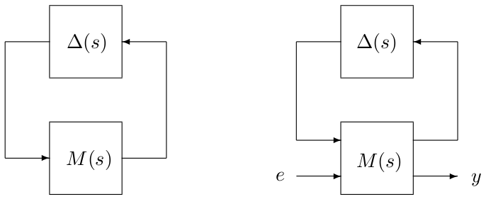
If $M(s)$ has no exogenous input and output, a robust stability problem is considered: a (skew-)$\mu$ lower bound, i.e. an upper bound $k_{ub}$ on the robustness margin $k_{max}$, is computed (see problem 1 on the overview page of the toolbox for more details). An associated destabilizing value $\tilde{\Delta}(s)$ of $\Delta(s)$ is also determined, and the considered stability region can be bounded either by the imaginary axis or by a truncated sector.

If $M(s)$ has exogenous inputs $e$ and outputs $y$, a worst-case $\mathcal{H}_\infty$ performance problem is considered: a lower bound $\gamma_{lb}$ is computed on the highest $\mathcal{H}_\infty$ norm $\gamma_{max}$ of the transfer matrix between $e$ and $y$ when $\Delta(s)$ takes any admissible value (see problem 2 on the overview page of the toolbox for more details). A value $\tilde{\Delta}(s)$ of $\Delta(s)$ for which the bound is obtained is also determined, and the $\mathcal{H}_\infty$ norm can be computing either along the imaginary axis or along the boundary of a truncated sector.

Note: In both cases, the initial interconnection is normalized with convert_data before the problem is solved.

Syntax

[lbnd,wc,pert,iodesc]=mulb(usys{,skew/perf,options}) [lbnd,wc,pert,iodesc]=mulb(gsys{,skew/perf,options}) [lbnd,wc,pert,iodesc]=mulb(lsys{,skew/perf,options}) [lbnd,wc,pert,iodesc]=mulb(sys,blk{,skew/perf,options})

Input arguments

The interconnection between $M(s)$ and $\Delta(s)$ can be described by:

a USS object usys,
a GSS object gsys,
a LFR object lsys,
a LTI object sys describing the LTI system $M(s)$ and a $N\times 2$ matrix blk defining the structure of the block-diagonal operator $\Delta(s)=diag\left(\Delta_1(s),\dots,\Delta_N(s)\right)$:
- blk(i,:)=[-ni 0] $\Rightarrow$ $\Delta_i(s)=\delta_iI_{n_i}$ with $\delta_i$ real,
- blk(i,:)=[ni 0] $\Rightarrow$ $\Delta_i(s)=\delta_iI_{n_i}$ with $\delta_i$ complex,
- blk(i,:)=[ni mi] $\Rightarrow$ $\Delta_i(s)$ is a $n_i\times m_i$ LTI system.

For a robust stability problem, an additional input argument skew can be defined, indicating whether the maximum admissible $\mathcal{H}_\infty$ norm of each $\Delta_i(s)$ is bounded (skew(i)=0) or not (skew(i)=1). If skew is undefined, skew(i) is set to 1 for all $i=1,\dots,N$, which means that a classical $\mu$ problem is considered.

For a worst-case $\mathcal{H}_\infty$ performance problem, an additional input argument perf can be defined to specify how the transfer between $e$ and $y$ is structured. Each line of perf corresponds to a performance channel. For example, if perf=[2 1;1 3], the transfer between inputs 1-2 and output 1 is considered independently of the one between input 3 and outputs 2-3-4. If perf is undefined, it is set to [ne ny], where ne and ny denote the size of the signals $e$ and $y$. The last input argument options is an optional structured variable with fields:

`freq`	Frequency interval $\Omega$ in rad/s on which the bound is to be computed. The default value is `options.freq=[0 10*max(abs(eig(sys)))]`.
`grid`	Frequency grid in rad/s ($1\times m$ array). It can also be a negative integer -$m$, in which case a $m$-point grid is automatically generated from $\Omega$. The default value is `options.grid=-10` if all uncertainties are real and `options.grid=-50` otherwise.
`sector`	Vector $[\alpha\ \xi]$ or $[\alpha\ \xi\ \omega_c]$ characterizing the considered truncated sector (see `display_sector` for a complete description). The default value is `options.sector=[0 0]`, which means that the left half plane is considered.
`target`	The algorithm is interrupted if a (skew-)$\mu$ lower bound or a lower bound on the worst-case $\mathcal{H}_\infty$ norm is found which is greater than `options.target`. The default value is `options.target=Inf`.
`trace`	Trace of execution. The default value is `options.trace=1`.
`warn`	Warnings display. The default value is `options.warn=1`.

Additional fields can be defined (see mulb_mixed, mulb_1real, mulb_nreal and hinflb_real), but the ones listed above are usually sufficient for non-expert users.

Output arguments

`lbnd`	Upper bound $k_{ub}$ on the robustness margin for the normalized interconnection, or lower bound $\gamma_{lb}$ on the worst-case $\mathcal{H}_\infty$ norm for each performance channel, on the considered frequency interval $\Omega$.
`wc`	Frequency $\omega_c$ in rad/s for which $k_{ub}$ or $\gamma_{lb}$ has been computed.
`pert`	The normalized interconnection is unstable (robust stability problem) or the $\mathcal{H}_\infty$ norm of the transfer between $e$ and $y$ is greater than or equal to $\gamma_{lb}$ (worst-case $\mathcal{H}_\infty$ performance problem) for every perturbation $\tilde{\Delta}(s)$ whose frequency response $\tilde{\Delta}(p(\omega_c))$ is equal to `pert`, where $p(\omega_c)$ denotes the point $j\omega_c$ on the imaginary axis or the corresponding point on the boundary of the truncated sector defined by `options.sector`.
`iodesc`	Cell array of structured variables: The name of the ith uncertainty $\Delta_i(s)$ is given by `iodesc{i}.name`. Its type is given by `iodesc{i}.type`: `'real scalar'` $\Rightarrow$ $\Delta_i(s)=\delta_iI_{n_i}$ with $\delta_i$ real, `'complex scalar'` $\Rightarrow$ $\Delta_i(s)=\delta_iI_{n_i}$ with $\delta_i$ complex, `'dynamical system'` $\Rightarrow$ $\Delta_i(s)$ is a $n_i\times m_i$ LTI system. The initial interconnection is unstable (robust stability problem) or the $\mathcal{H}_\infty$ norm of the transfer between $e$ and $y$ is greater than or equal to $\gamma_{lb}$ (worst-case $\mathcal{H}_\infty$ performance problem) for every perturbation $\tilde{\Delta}(s)$ whose frequency response $\tilde{\Delta}(p(\omega_c))$ is defined as follows: $\tilde{\delta}_i=$`iodesc{i}.value` if `iodesc{i}.type='real scalar'` or `'complex scalar'`, $\tilde{\Delta}_i(p(\omega_c))=$`iodesc{i}.value` if `iodesc{i}.type='dynamical system'`. In case a worst-case $\mathcal{H}_\infty$ performance problem is considered, the last cell of `iodesc` is associated to the performance channels. In this case, `iodesc{end}.name=''`, `iodesc{end}.type='performance channel'` and `iodesc{end}.norm` contains the lower bound $\gamma_{lb}$ on the worst-case $\mathcal{H}_\infty$ norm for each performance channel.

Example

1. Robust stability problem

Description of the uncertain system by a USS object:
a1=ureal('a',5,'Percentage',20);
b1=ucomplex('b',4+3*sqrt(-1),'Percentage',40);
c1=ultidyn('c',[2 1],'Bound',2,'Type','GainBounded');
A1=[-3*a1*b1-2 1;a1 -b1^2-1]+c1*[a1 -b1];
usys=lft(tf({1 0;0 1},[1 0]),A1);
usys=simplify(usys,'full');
Computation of an upper bound $k_{ub}$ on the robustness margin $k_{max}$ for the normalized interconnection:
lbnd1,wc1,pert1,iodesc1]=mulb(usys);
k_ub=1/lbnd1
Frequency response $\tilde{\Delta}(\omega_c)$ of a perturbation $\tilde{\Delta}(s)$ which makes the initial interconnection unstable: iodesc1{:} sys1=usubs(usys,'a',iodesc1{1}.value,'b',iodesc1{2}.value,'c',iodesc1{3}.value); damp(sys1)

Description of the uncertain system by a GSS object:
a3=gss('a',5,[4 6]);
b3=gss('b',4+3i,[4 3 2]);
c3=gss('c','LTI',[2 1],0,2);
A3=[-3*a3*b3-2 1;a3 -b3^2-1]+c3*[a3 -b3];
gsys=abcd2gss(A3,2);
Computation of an upper bound $k_{ub}$ on the robustness margin $k_{max}$ for the normalized interconnection:
lbnd3,wc3,pert3,iodesc3]=mulb(gsys);
k_ub=1/lbnd3
Frequency response $\tilde{\Delta}(\omega_c)$ of a perturbation $\tilde{\Delta}(s)$ which makes the initial interconnection unstable: iodesc3{:}
sys3=eval(gsys,{'a' 'b' 'c'},{iodesc3{2}.value iodesc3{3}.value iodesc3{1}.value}); damp(sys3)

2. Worst-case $\mathcal{H}_\infty$ performance problem

Description of the uncertain system by a LFR object:
a2=lfr('a','ltisr',1,[4 6],'minmax');
b2=lfr('b','ltisc',1,[4+3*sqrt(-1) 2],'disc');
c2=lfr('c','ltifc',[2 1],ltisys([],[],[],2),'freq');
d2=lfr('d','ltifc',[2 2],ltisys(-1,1,3,2),'freq');
A2=[-3*a2*b2-2 1;a2 -b2^2-1]+c2*[a2 -b2];
B2=[1 3;2 a2];
C2=d2*[b2 1;2 -3];
D2=[0 2;0 1];
lsys=abcd2lfr([A2 B2;C2 D2],2);
lsys=minlfr(lsys);
size(lsys)
Computation of a lower bound $\gamma_{lb}$ on the worst-case $\mathcal{H}_\infty$ norm $\gamma_{max}$: [lbnd2,wc2,pert2,iodesc2]=mulb(lsys);
gamma_lb=lbnd2
Frequency response $\tilde{\Delta}(\omega_c)$ of a perturbation $\tilde{\Delta}(s)$ for which the $\mathcal{H}_\infty$ norm or the initial interconnection is equal to $\gamma_{lb}$: iodesc2{:}
a=iodesc2{1}.value;b=iodesc2{2}.value;c=iodesc2{3}.value;d=iodesc2{4}.value;
sys2=eval(lsys);
svd(calc_freq_resp(ss(sys2.a,sys2.b,sys2.c,sys2.d),wc2,[0 0]))

Description

Syntax

Input arguments

Output arguments

Example

See also