Routine mubb_mixed

Compute (skew-)$\mu$ upper and lower bounds with desired accuracy for mixed perturbations.

Description

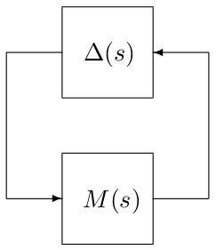
This routine computes both (skew-)$\mu$ upper and lower bounds for an interconnection between a nominal LTI system $M(s)$ and a block-diagonal operator $\Delta(s)= diag\left(\Delta_1(s),\dots,\Delta_N(s)\right)$. A branch and bound scheme is implemented: the real parametric domain is partitioned in more and more subsets until the highest lower bound lbnd and the highest upper bound ubnd computed on all subsets satisfy ubnd$\,\le$(1+maxgap)*lbnd, where maxgap is a user-defined thresohld. The considered stability region can be bounded either by the imaginary axis or by a truncated sector.

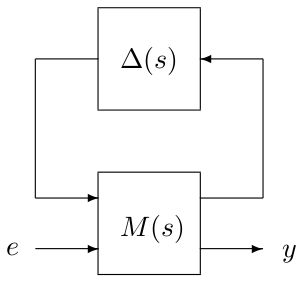
This routine can also be used to solve a worst-case $\mathcal{H}_\infty$ performance problem, which is nothing but a specific skew-$\mu$ problem. A fictitious stable and proper real-rational unstructured transfer matrix is just added between the output $y$ and the input $e$. An example is given at the bottom of this page. In this case, the output argument bnds contains lower and upper bounds on the worst-case $\mathcal{H}_\infty$ norm of the transfer matrix from $e$ to $y$.

Warning: This algorithm always converges for systems with only real uncertainties, even if maxgap is chosen arbitrarily small. Note however that maxgap allows to handle the tradeoff between accuracy and computational complexity, and that very small values can sometimes lead to prohibitive computational times. Moreover, the algorithm usually exhibits an exponential growth of computational complexity as a function of the number of real uncertainties. In this context, the $\mu$-sensitivities can be used to get the same accuracy with a reduced number of iterations (see options.musen).

Syntax

[bnds,wc,pert,tab,elts]=mubb_mixed(sys,blk{,options})

Input arguments

The first two input arguments are mandatory:

sys LTI object describing the nominal system $M(s)$.

blk

Matrix defining the structure of the block-diagonal operator $\Delta(s)=diag\left(\Delta_1(s),...,\Delta_N(s)\right)$. Its first 2 columns must be defined as follows for all $i=1,...,N$:

blk(i,1:2)=[-ni 0] $\Rightarrow$ $\Delta_i(s)=\delta_iI_{n_i}$ with $\delta_i$ real,
blk(i,1:2)=[ni 0] $\Rightarrow$ $\Delta_i(s)=\delta_iI_{n_i}$ with $\delta_i$ complex,
blk(i,1:2)=[ni ni] $\Rightarrow$ $\Delta_i(s)$ is a $n_i\times n_i$ LTI system.

A third column can be used to specify skew uncertainties:

blk(i,3)=0 $\Rightarrow$ $\overline{\sigma}(\Delta_i(j\omega))\le 1$ for all $\omega\in\Omega$,
blk(i,3)=1 $\Rightarrow$ $\overline{\sigma}(\Delta_i(j\omega))$ is unconstrained for all $\omega\in\Omega$.

If none, blk(i,3) is set to 1 for all $i=1,...,N$.

The third input argument options is an optional structured variable with fields:

`maxgap`	Maximum gap between the bounds. The default value is `options.maxgap=0.05`, i.e. 5%. In case of a $\mu$-test, (`options.umax>0`), `options.maxgap` is used to set `options.tol` in `muub_mixed`.
`maxcut`	Maximum number of times the real parametric domain can be bisected. The default value is `options.maxcut=100`.
`maxtime`	Maximum computational time. The default value is `options.maxtime=Inf`.
`musen`	If `options.musen=0`, the parametric domain is always bisected along its longest edge (classical branch and bound algorithm). If `options.musen=Inf`, the parametric domain is always bisected along the edge with the highest mu-sensitivity. If `options.musen=m` is a strictly positive integer, the algorithm switches between the two strategies every m iterations in case of slow progress.The default value is `options.musen=10`.
`freq`	Frequency interval $\Omega$ in rad/s on which the bounds are to be computed. The default value is `options.freq=[0 10*max(abs(eig(sys)))]`.
`sector`	Vector $[\alpha\ \xi]$ or $[\alpha\ \xi\ \omega_c]$ characterizing the considered truncated sector (see `display_sector` for a complete description). The default value is `options.sector=[0 0]`, which means that the left half plane is considered.
`trace`	Trace of execution. The default value is `options.trace=1`. An `'s'` in the first column indicates that the $\mu$-sensitivities have been used.
`warn`	Warnings display. The default value is `options.warn=1`.
`umax`	If nonzero, the algorithm checks whether the (skew-)$\mu$ upper bound is less than `options.umax` ($\mu$-test). In this case, no lower bound is computed. The default value is `options.umax=0`.

Additional fields can be defined if necessary: lmi, reg, maxiter for upper bound computation (see muub_mixed) ; method, improve, grid for lower bound computation (see mulb_mixed or mulb_nreal).

Output arguments

`bnds`	(Skew-)$\mu$ lower and upper bounds `lbnd` and `ubnd` on the considered frequency interval $\Omega$. `ubnd` is valid only if the algorithm succeeds, i.e. if `elts.invalid` is empty.
`wc`	Frequency $\omega_c$ in rad/s for which `lbnd` has been computed.
`pert`	Unless `lbnd=0`, every perturbation $\tilde{\Delta}(s)$ whose frequency response $\tilde{\Delta}(\omega_c)$ at $j\omega_c$ (or at the corresponding point on the boundary of the truncated sector defined by `options.sector`) is equal to `pert` satisfies $\mbox{det}(I-M(\omega_c)\tilde{\Delta}(\omega_c))\approx 0$, where $M(\omega_c)$ is the frequency response of $M(s)$.
`tab`	Structured variable with fields: `lbnd`: other (skew-)$\mu$ lower bounds ($m\times 1$ array). `wc`: associated frequencies in rad/s ($m\times 1$ array). `pert`: associated destabilizing perturbations ($n\times n\times m$ array, where $n=\displaystyle\sum_{i=1}^{N}{n_i}$).
`elts`	Structured variable with fields `valid` and `invalid`: `elts.valid(k)` describes the kth validated subset and is composed of fields: `freq`: frequency interval. `domain`: real parametric domain (one line per parameter). `ncut`: number of bisections needed to obtain the subset. `utest`: upper bound considered during validation. `elts.invalid(k)` describes the kth invalidated subset and is composed of the same fields as `elts.valid(k)`. It is empty if the algorithm succeeds.

Examples

1. Classical $\mu$ problem

System with 60 states and 3 repeated uncertainties:
minz=1;
alpha=0;
while minz>0.03 || alpha>-0.25
$\ \ \ $ sys=rss(60,30,30)/100;
$\ \ \ $ [om,z]=damp(sys);
$\ \ \ $ minz=min(z);
$\ \ \ $ alpha=max(real(eig(sys)));
end
blk=[-10 0;-15 0;-5 0];

Computation of upper and lower bounds:
[ubnd,wc,tab]=muub_mixed(sys,blk);
[lbnd,wc,pert]=mulb_nreal(sys,blk);
100*(ubnd/lbnd-1)
The gap between the bounds is quite large.

Computation of upper and lower bounds with desired accuracy:
options.maxgap=0.01;
[bnds,wc,pert,tab,elts]=mubb_mixed(sys,blk,options);
The computational time is higher but the gap is now only 1%.

2. Worst-case $\mathcal{H}_\infty$ performance problem

System with 60 states and 2 repeated uncertainties, which are both kept inside the unit ball. The third block of $\Delta(s)$ corresponds to the performance channel:
blk=[-10 0 0;-15 0 0;5 5 1];
[bnds,wc,pert,tab,elts]=mubb_mixed(sys,blk,options);

Reference