Example

The following results have been obtained with Matlab 2012b, Windows 7 64bits, an Intel(R) Xeon(R) CPU W3530 @2.80GHz and 6.00 Go of RAM. For more details reader can refer to the user's guide.

Military aircraft model

The objective is to analyze the closed loop stability. This closed loop corresponds to the interconnection of a military aircraft model with a control law. In this analysis problem we have to consider:

• One critical static non-linearity which corresponds to a rate limiter. This rate limiter has been transformed into a normalized dead zone;
• Two LPV parameters which correspond to the mach number and the calibrated airspeed with a nominal rate of variation of 0.2 for both. These two time-varying parameters represent the flight case. The mach number and the calibrated airspeed respectively vary from 0 to 1 and from 150 to 275 kts.
• Five real LTI uncertainties. These real uncertainties are combination of different physical real uncertainties as mass, center of gravity position etc... This transformation is necessary to obtain a limited size for the LFT model. But the important think to keep in mind is the stability analysis is done for the maximum variation of real uncertainties and not a for restricted domain. In other words if the stability is guaranteed with all LTI uncertainties, the stability is guaranteed for the whole domain of physical parameters.

The structure of $\Delta$ is the following one:

• One (0,1) sector non-linearity is considered;
• The Mach number is repeated twice;
• The calibrated airspeed is repeated eight times;
• Each real uncertainty is repeated once;
• Finally the number of inputs/outputs of $\Delta$ is sixteen.

The multipliers dynamic is a first order low-pass filter with a pole at 10 rad/s. The initial frequency griding is $\omega_i=\{1,5,10,20,100\}$ $rad/s$ with $i=1,...,5$. A 310 decision variables feasibility problem is solved. Finally the result has been obtained in 3 iterations and $250$ $s$.

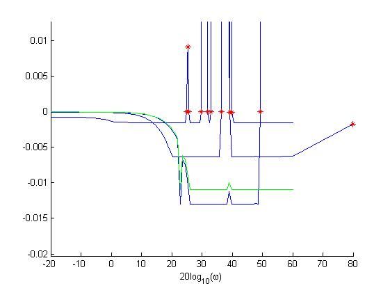
Figure 1: Iterative representation of the stability criterion

Figure 2: The final stability criterion

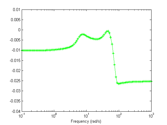
In Figure 1 the equivalent stability criterion (1), named $\Xi(s)$, obtained by the bilinear transformation $\frac{Z-1}{Z+1}$ has been represented at each iteration. The green line represents the final solution which satisfies the weak gain condition. The red stars represent the critical frequencies which are added iteratively. In brief for each frequency domain where the stability criterion is not valid three frequencies are added. Two frequencies correspond to frequencies where the stability criterion intercepts the $x$ ax and the last one corresponds to an intermediate frequency . For more details please refer to the user's guide. Finally Figure 2 represents the real and negative eigenvalues of the final stability criterion.

Figure 3: The stability criterion for each iteration

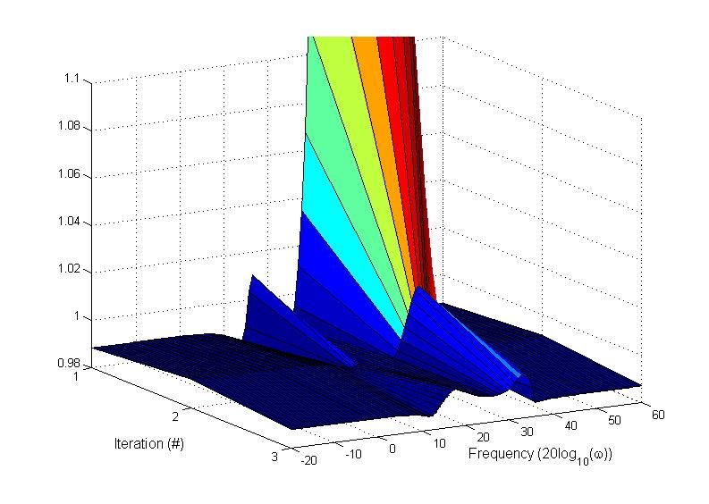
A 3D representation is given by Figure 3.

High dimensional civil aircraft aeroelastic model

An aeroelastic model with two freeplays on elevators has been considered. This model is characteristic of aeroelastic models used for load level evaluation or stability analysis. The main idea is to separate the condensed structural non-linearities from the rest of the linear aircraft model. The aeroelastic equation is written for the linear part, i.e. for the aircraft in nominal configuration except for its control surfaces (two elevators in our study), which are connected at their hinges but have no stiffness in rotation. Thus the resulting modal basis includes the rotation modes of both elevators which are at zero frequency. For each elevator, the non-linearity is modeled as external force, applied between its attachments. Then both linear and non-linear models are linked via the relative displacement of the attachments and the actuator forces. The study of the non-linear aeroelastic model can be viewed as a problem of closed loop with a linear part which corresponds to the linear aeroelastic model, interconnected to the static non-linearities which correspond to the freeplays.

To limit the computational effort for the frequency domain validation step, it is interesting to reduce the order of G(s). In brief the optimization problem is independent from the order of G(s) but the validation step is based on matrix eigenvalues whose the size depends on G(s) order. To ensure stability on the full order model a frequency domain error between the full and the reduced model is modelled. This error is seen as a neglected dynamic represented by $\Delta(s)$. Finally G(s) is the linear part seen by the block $\Delta$. G has four inputs/outputs which correspond to inputs/outputs of static non-linearities and $\Delta$ block. To reduce the model order a very classical approach has been involved. This one is based on Gramian-based balancing of state-space realizations. More precisely for stable systems, a balanced realization is a state space representation for which the controllability and observability gramians are equal and diagonal. When this representation is obtained, the states with the lowest controllability/observability gramians are considered as negligible and then are eliminated. The full order aeroelastic model is of order 550. Finally a reduced order model of order 152 is obtained.

The final objective is to prove the stability with the two non-linearities on the full order model [6]. As indicated previously this is done by considering the reduced order model with two non-linearities combined with the frequency domain reduction error $\Delta(s)$. The results are obtained in 9 seconds since finally the number of optimization variables is very limited in spite of the order of the reduced aeroelastic model $(=152)$. With the KYP lemma it is necessary to add optimization variables of $P$. For $P$ we have $(n^2+n)/2$ variables where $n$ corresponds to the order of the augmented system, i.e. 160. In brief the number of decision variables is equal to 12889, i.e. 12880 from $P$ + 9 from $M$ (which is slightly different from [6] since here Park multiplier is involved). Either the problem is untractable or the resolution time is unacceptable. Even if it is possible to reduce the order of the reduced model to 50 for example, with a larger $\Delta(s)$, the number of decision variables is high and the state space approach remains outperformed by the frequency domain resolution. And it is important to keep in mind that it is rarely possible to have an order inferior to 50 for an aeroelastic model of a large civil aircraft.

The initial frequency domain griding is $\omega_0=1,5,10, 20, 100$ $rad/s$. The result is obtained in $9$ $s$ and $4$ iterations.
The maximum singular value of $\Xi(s)$ is represented at each iteration by Figure 4.

Figure 4: The iterative representation of the stability criterion for an high dimensional aeroelastic model