Routine lsapprox

Polynomial approximation of tabulated data using linear least-squares.

Description

This routine uses Linear Least-Squares to compute a multivariate polynomial approximation f : ℝⁿ→ ℝⁿ_¹^×n_² of a set of samples { y_k∈ ℝⁿ_¹^×n_², k ∈ [1, N] } obtained for different values { x_k ∈ ℝⁿ, k ∈ [1, N]} of some explanatory variables x ∈ ℝⁿ. The maximum degree of the polynomial function is set by the user. No maximum admissible error can be specified and a full polynomial expression is obtained, which minimizes the global relative error and the root-mean-square error between { f(x_k), k ∈ [1, N]} and {y_k, k ∈ [1, N]} for each entry (see errapprox for precise definitions).

Syntax

[fdata,flfr]=lsapprox(X,Y,names,maxdeg{,options})

Input arguments

The first four input arguments are mandatory:

`X`	Values $\left\{x_k\in\mathbb{R}^n,k \in [1, N]\right\}$ of the explanatory variables $x$ ($n\times N$ array, where `X(:,k)` corresponds to $x_k$).
`Y`	Samples $\left\{y_k\in\mathbb{R}^{n_1\times n_2}, k\in [1, N]\right\}$ to be approximated ($n_1\times n_2\times N$ array where `Y(:,:,k)` corresponds to $y_k$ in the general case, or possibly $1\times N$ array where `Y(k)` corresponds to $y_k$ if $n_1=n_2=1$).
`names`	Names of the explanatory variables $x$ ($1\times n$ cell array of strings).
`maxdeg`	Maximum degree of the approximating polynomial function $f$.

The fifth input argument options is an optional structured variable with fields:

`maxexp`	Maximum exponent of each explanatory variable in the approximating polynomial function $f$ ($1\times n$ array). The default value is `options.maxexp=maxdeg*ones(1,n)`.
`Xeq` `Yeq`	Constraint to be exactly met (no least squares). `options.Yeq` is a $n_1\times n_2$ array and `options.Xeq` is a $n\times 1$ vector with associated values of the explanatory variables. The default values are `options.Xeq=[]` and `options.Yeq=[]`.
`trace`	Trace of execution (0=no, 1=text, 2=text+figures). The default value is `options.trace=1`.
`viewpoint`	This option is applicable only if 3-D graphs are to be displayed (`options.trace=2` and n=2). It represents the deviation with respect to the default viewpoint (see `plotapprox`). The default value is `options.viewpoint=[0 0]`.

Output arguments

`fdata`	Values $\left\{f(x_k)\in\mathbb{R}^{n_1\times n_2},k \in [1, N]\right\}$ of the approximating function $f$ (same size as `Y`).
`flfr`	Linear fractional representation of the approximating function $f$ (GSS object if the GSS library is installed, LFR object otherwise if the LFR toolbox is installed).

Caution

If some values in X are much larger than 1, they must be scaled or normalized.

Example

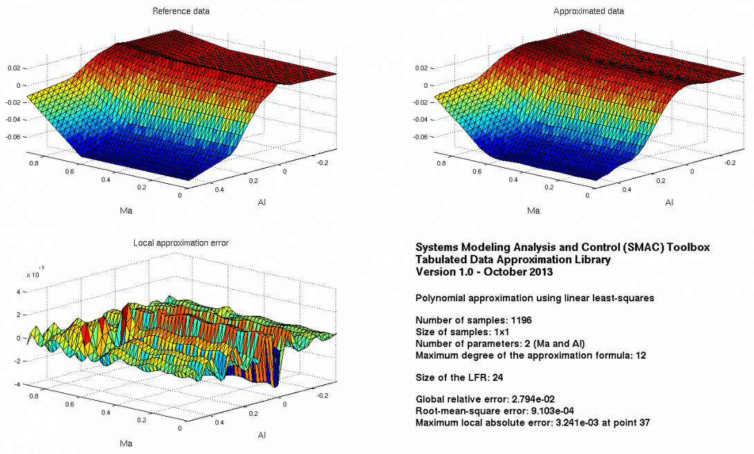
Drag coefficient of a generic fighter aircraft model:
load data_cx
Approximation on a rough grid:
maxdeg=12;
options.trace=2;
options.viewpoint=[-100 0];
[fdata,flfr]=lsapprox(X1,Y1,names,maxdeg,options);

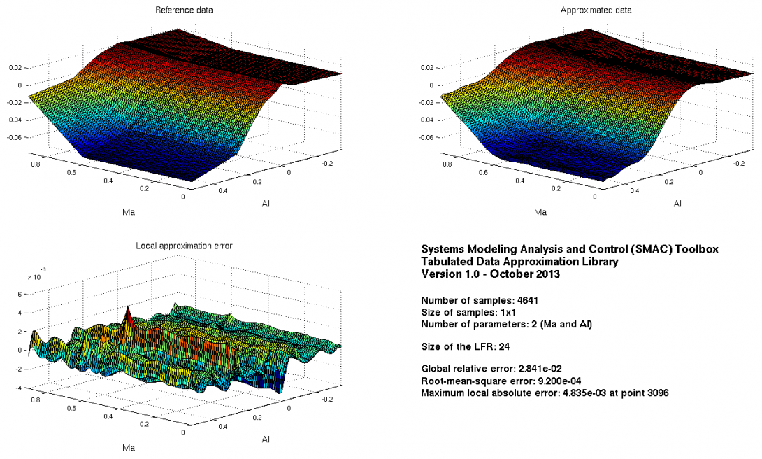
Validation on a fine grid:
plotapprox(Xv,Yv,names,flfr,options);

References

[1]	C. Poussot-Vassal and C. Roos, "Generation of a reduced-order LPV/LFT model from a set of large-scale MIMO LTI flexible aircraft models", Control Engineering Practice, vol. 20, no. 9, pp.919-930, 2012.
[2]	C. Roos, "Generation of LFRs for a flexible aircraft model", Optimization based clearance of flight control laws, Lecture Notes in Control and Information Sciences, vol. 416, pp. 59–77, Springer Verlag, 2011.