Rational approximation of tabulated data using genetic programming.
Description
This routine uses Genetic Programming (see below) to compute a multivariate rational approximation $f:\mathbb{R}^n\rightarrow\mathbb{R}$ of a set of scalar samples $\left\{y_k\in\mathbb{R}, k\in [1, N]\right\}$ obtained for different values $\left\{x_k\in\mathbb{R}^n,k \in [1, N]\right\}$ of some explanatory variables $x$. The maximum degree of the rational function is set by the user and a sparse rational expression is usually obtained. Unless specified, its nonsingularity is guaranteed on the whole considered domain (defined as the convex hull of $\left\{x_k\in\mathbb{R}^n,k \in [1, N]\right\}$).
When the model structure has to be determined as a whole (numerator/denominator degrees, number and type of monomials), the problem cannot generally be solved by means of classical techniques. Over a few explanatory variables, a sequential and systematic exploration of the terms cannot reasonably be expected owing to the curse of dimensionality. E.g., for 2 variables and a maximum degree of 10, there are not less than $10^{15}$ rational candidates available! Moreover, this dual-purpose optimization (model structure and parameters) is complicated by the fact that a rational model is no more a Linear-in-its-Parameters (LP) model. Happily, some promising techniques have recently appeared for global optimization, with the purpose of solving symbolic regression problems close to this one. It is especially the case of Genetic Programming and that is why this was adapted to the approximation of a rational function. The interest in combining least-squares methods (LS) with symbolic optimization of the kernel functions has already been studied some years ago and has resulted for instance in the Matlab code GP-OLS [4]. More recently, another Toolbox has been developed (GPTIPS), permitting to encode and to adapt a LP model in a multigene symbolic regression form [6]. However, none of those tools is suitable for directly synthetizing a rational modeling, especially because the parameter optimization becomes a nonlinear process then.
Consequently, the approach proposed here is somewhat different and is dedicated to the rational case. It is issued from several considerations: 1/ the rational case extends the polynomial case (structured modeling expressed as the quotient of two polynomials) 2/ GP is fully justified then since there is no other classical option available for jointly optimizing the structure of numerator and denominator (a brute-force search would not attempt to minimize the number of monomials) 3/ those two components remain LP when considered separately, and it would be a pity not to take advantage of that. In other words, GP is clearly a promising alternative for rational modeling, but a prior adaptation of the method is required to use it with a maximum efficiency. That is why the algorithm called TRACKER (Toolbox for Rational Approximation Computed by Knowing Evolutionary Research) has been developed by ONERA. See [2] for more details.
TRACKER algorithm in a few words
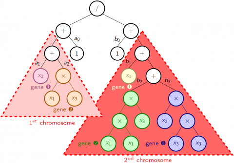
The outlines of TRACKER are the following [2]. Each component of the rational function (numerator and denominator) is represented by a single separate chromosome which comes in a syntax tree form as usual, and a priori includes several genes. The sets F$=\{+,*\}$ and T$=\{x^0=1,x^1,...,x^n\}$ are chosen as for the polynomial case (see section below about GP), and a peculiar syntax rule is defined to ensure that all the non terminal nodes located below a "$*$"-type node are also "$*$"-type nodes. This trick avoids to create useless branching which could result in splitting and multiplying some monomials. Thanks to this architecture, a gene appears as a subtree linked to the root node of its chromosome through one or several "$+$"-type nodes. A parse analysis of the different genes composing a chromosome also permits to avoid the creation of spurious genes by identifying and grouping them if any. As an example, the figure below depicts the tree's architecture corresponding to the function $(a_0+a_1*x_2+a_2*x_1*x_3)/(b_0+b_1*x_1+b_2*x_1^2*x_3+b_3*x_2*x_3^2)$. The 5 genes related to the different monomials are highlighted by colours (except from the constants $a_0$ and $b_0$ which are an integral part of the structure).
To solve the parametric optimization, i.e. to estimate the regression coefficients $(a_j,b_j)$ of any created tree, TRACKER implements a well-known technique, in use for identifying transfer functions in the frequency domain [1,5]. In the general case where $f$ is a rational function expressed as:
$(2)\hspace{2cm}y_k=f(x_k)=P(x_k)\bigg/Q(x_k)=\displaystyle\sum_{j=0}^{n_P}a_j\ r_j^P(x_k)\bigg/\displaystyle\sum_{j=0}^{n_Q}b_j\ r_j^Q(x_k)$
where $\left\{r_j^P,j\in [1,n_P]\right\}$ and $\left\{r_j^Q,j\in [1,n_Q]\right\}$ are two sets of monomial regressors, this consists in iteratively linearizing the expression of the error term involved in the quadratic cost function as:
$(3)\hspace{2cm}\hat{\epsilon}_k\simeq\bigg[\displaystyle\sum_{j=0}^{n_P}a_j\ r_j^P(x_k)-\displaystyle\sum_{j=1}^{n_Q}b_j\ y_k\ r_j^Q(x_k)-y_k\bigg]\bigg/\bigg[1+\displaystyle\sum_{j=1}^{n_Q}\hat{b}_j\ r_j^Q(x_k)\bigg]$
where the approximation of $\epsilon_k$ comes from the replacement of the parameters $b_j$ by their most recent estimates $\hat{b}_j$ at the running iteration, and the denominator is arbitrarily normalized by choosing $b_0=1$. This algorithm relies on the fact that the denominator approximation becomes fully justified when the iterative process has converged. Hence, the parameters $(a_j,b_j)$ to be determined just become solution of a linearized LS problem. In practice, 2 or 3 iterations are usually sufficient to ensure the convergence of this process, conveniently initialized by setting the denominator to 1 at the first iteration. In case of ill-conditioning, a few iterations of Levenberg-Marquardt optimization are used to recover a satisfactory result. Introduced into the GP selection process (see section below about GP), that technique enables to evaluate the performance of every individual very easily, by coming down to a short series of ordinary LS. The overcost remains limited because the major part of the computations required for the regression matrix can be stored and reused throughout the loop. Otherwise, to get well-defined LFRs, an important issue is to check that the denominator has no roots in the considered domain, i.e. $Q(x)\neq0$ for all $x$. Hence, a $\mu$-analysis based technique is implemented to check the nonsingularity of the resulting functions, and additional constraints are introduced until strictly positive denominators are obtained [2].
Syntax
[pop,best,fdata,fdesc,fsym,flfr]=tracker(X,Y,names,maxdeg{,options})
Input arguments
The first four input arguments are mandatory:
X | Values $\left\{x_k\in\mathbb{R}^n,k \in [1, N]\right\}$ of the explanatory variables $x$ ($n\times N$ array, where X(:,k) corresponds to $x_k$). |
Y | Samples $\left\{y_k\in\mathbb{R}, k\in [1, N]\right\}$ to be approximated ($1\times N$ array where Y(k) corresponds to $y_k$). |
names | Names of the explanatory variables $x$ ($1\times n$ cell array of strings). |
maxdeg | Maximum degree of the approximating rational function $f$. |
The fifth input argument is an optional structured variable. Default values are given between brackets. Most of the parameters can be left to their default setting, some of them (tree features, evolutionary process) being especially devoted to experienced users. The most important ones are maxexp, nbind and nbgen.
options | $\hspace{0.65cm}$User constraints and settings
|
Output arguments
pop | Structure containing the main information about the individuals of the final population:
|
best | Index of the best individual in the final population (with respect to fitness). |
fdata | Values $\left\{f(x_k)\in\mathbb{R}, k \in [1, N]\right\}$ of the approximating function $f$ corresponding to the best individual (same size as Y). |
fdesc | Description of the approximating function $f$ corresponding to the best individual (fdesc.cnum(j)/cden(j) and fdesc.enum(j,:)/eden(j,:) contain the coefficient and the exponents of the $j$th monomial of the numerator/denominator used to approximate Y). |
fsym | Symbolic representation of the rational function $f$ corresponding to the best individual (symbolic object). |
flfr | Linear fractional representation of the rational function $f$ corresponding to the best individual (GSS object if the GSS library is installed, LFR object otherwise if the LFR toolbox is installed). |
See also
lsapproxolsapproxqpapproxkoala
Example
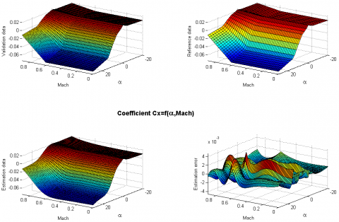
Drag coefficient of a generic fighter aircraft model:load data_cx% alfa angle converted from radians to degrees (estimation and validation data)X1(2,:)=X1(2,:)*57.3;Xv(2,:)=Xv(2,:)*57.3;% approximation on a rough gridmaxdeg=8;pop,best,fdata,fdesc,fsym,flfr]=tracker(X1,Y1,names,maxdeg,tracker_options);
----------------------------------------------------------------------
Systems Modeling Analysis and Control (SMAC) Toolbox
APRICOT Library Version 1.0 - April 2014
Rational approximation using Genetic Programming
----------------------------------------------------------------------
Number of samples: 1196
Number of explanatory variables: 2
Creation of 4 fictitious variables
- with degrees w.r.t. explanatory variable #1: 3 5
- with degrees w.r.t. explanatory variable #2: 3 5
Maximum degree required for the approximation function: 8
Maximum degree required for each variable: 8 8
The population is comprised of 100 individuals and will be evolved over 100 generations at most
There are 6 explanatory variables, including 4 fictitious variables (added to get simpler trees)
Generation 0 --> best fitness: 0.00283915 (40 nodes)
Generation 5 --> best fitness: 0.00118514 (76 nodes)
Generation 10 --> best fitness: 0.00118290 (72 nodes)
Generation 15 --> best fitness: 0.00115280 (84 nodes)
Generation 20 --> best fitness: 0.00111282 (80 nodes)
Generation 25 --> best fitness: 0.00104232 (88 nodes)
Generation 30 --> best fitness: 0.00104232 (88 nodes)
Generation 35 --> best fitness: 0.00102940 (84 nodes)
Generation 40 --> best fitness: 0.00099021 (86 nodes)
Generation 45 --> best fitness: 0.00099021 (86 nodes)
Generation 50 --> best fitness: 0.00095285 (84 nodes)
Generation 55 --> best fitness: 0.00094642 (98 nodes)
Generation 60 --> best fitness: 0.00094455 (96 nodes)
Generation 65 --> best fitness: 0.00092366 (102 nodes)
Generation 70 --> best fitness: 0.00092366 (102 nodes)
Generation 75 --> best fitness: 0.00092279 (100 nodes)
Generation 80 --> best fitness: 0.00092279 (100 nodes)
Generation 85 --> best fitness: 0.00092257 (94 nodes)
Generation 90 --> best fitness: 0.00078144 (98 nodes)
Generation 95 --> best fitness: 0.00078144 (98 nodes)
Final size of the archive memory: 8615
Positivity check is successful, everything is OK
Fitness value of the best individual #96: 0.00078144 (98 nodes)
Symbolic expression of the rational approximation
Numerator:0.0166278+0.00254291*Al^2+6.86357e-006*Al^4-0.000493197*Ma^4*Al^3+7.49538e-005*Ma^3*Al^3
+3.73923e-005*Ma*Al^3-5.59117e-006*Ma*Al^4-6.15747*Ma^4+3.6731e-005*Ma^3*Al^4-0.000507616*Al^3
-0.0793195*Ma+5.21629*Ma^5+2.02358*Ma^3-5.4279e-007*Al^5
Denominator: 1.0-16.6575*Ma^2+0.0972086*Ma^5*Al^3+0.261167*Al^2-235.275*Ma^6+0.00194204*Al^4
-0.073906*Ma^4*Al^3+0.00353226*Ma*Al^3-7.47814e-005*Ma*Al^4-697.819*Ma^4-0.0344331*Al^3+231.866*Ma^3
+0.141067*Al-2.48184e-005*Al^5-3.96694*Ma+765.611*Ma^5
Size of the LFR: (trial#1 --> 15 / trial#2 --> 20 / trial#3 --> 15) ==> Minimum size = 15
CPU time for the tracker call = 854 seconds
% Plot 3D surfaces (estimation results on a rough grid and validation results on a fine grid) plosurfs(pop,best,X1,Y1,names,Xv,Yv);
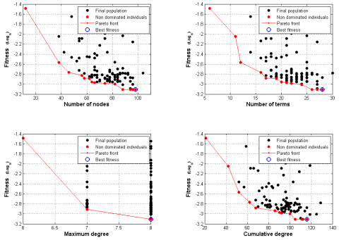
Individual #96 (98 nodes/28 terms/max degree 8/total degree 116)
Validation errors: Global=3.384660e-003 - RMS=8.539880e-004 - Max Local=4.596582e-003
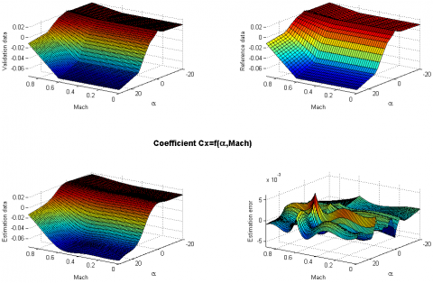
% Plot Pareto frontsplofronts(pop,best);% User loop to analyse and plot any individual (Pareto optimal solution)loop=1;while loopindiv = input('\nIndividual to be displayed (press RETURN to terminate) ?');if isempty(indiv)loop=0;elseplosurfs(pop,indiv,X1,Y1,names,Xv,Yv); [fdata,fdesc,fsym,flfr]=pop2lfr(pop,indiv,names,X1); endend
>>Individual to be displayed (press RETURN to terminate) ? 32
Individual #32 (66 nodes/21 terms/max degree 8/total degree 90)
Validation errors: Global=5.193755e-003 - RMS=1.057876e-003 - Max Local=6.213335e-003
Symbolic expression of the rational approximation
Numerator:0.0136579-2.66819e-010*Al^6+1.0892e-006*Al^4-0.0020092*Ma^4*Al^3+0.000711613*Ma^3*Al^3
+0.00136296*Ma^5*Al^3-0.000451564*Ma+0.202329*Ma^5-0.0670935*Ma^3-0.000739199*Al-5.0639e-005*Al^3
-3.52304e-008*Al^5
Denominator:1.0+0.0217883*Al^2+0.000157657*Al^4+0.00771755*Ma^5*Al^3-0.00226182*Ma^3*Al^3
-4.24916e-006*Ma*Al^4+11.9683*Ma^4-0.00272452*Al^3-0.368659*Ma-6.21157*Ma^3-2.14231e-006*Al^5 Size of the LFR: (trial#1 --> 16 / trial#2 --> 18 / trial#3 --> 16) ==> Minimum size = 16
$\Rightarrow$ the science of LFR sizes is not an exact one, ...and is often disappointing !!!
What is Genetic Programming ?
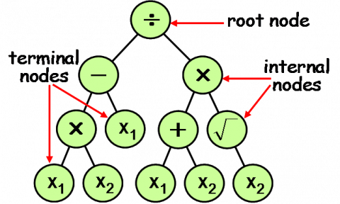
Genetic Programming (GP) is part of the evolutionary algorithms family, in the same way as GAs, evolutionary programming, etc. It uses the same principles inspired by those of natural evolution to evolve a population of individuals randomly created, improving its behavior progressively until a satisfactory solution is found. However, opposite to GAs, it is not based on a binary coding of information but uses a structured representation instead, as syntax trees. These parse trees appear more suited to solve structural or symbolic optimization problems since they can have different sizes and shapes. The alphabet used to create these models is also flexible enough to cope with different types of problems, and so they can be used to encode mathematical equations as well as behavior models, ... and even computer programs. First works date back to the early sixties, but GP was really implemented and brought up to date only in the early 90s by John Koza, thanks also to an increase of computing power. He was thus able to prove the interest of GP in many application fields, and laid the foundations of a standard paradigm which did not evolve much since then [3]. The iterative process, which breeds a population of programs, transforms them generation after generation by applying genetic mechanisms like those of Darwinian evolution: reproduction, mutation, crossover, but also gene duplication or deletion. Unlike GAs, they are applied to the hierarchically structured trees of the individuals, which comprise a set of nodes and links. These elements fall into two categories: the set F of internal nodes called functions or operators, and the set T of tree's leaves called terminals. An example is given below, corresponding to the mathematical function $f(x_1,x_2)=x_1(x_2-1)/(x_1+x_2)/\sqrt{x_2}$.
All types of functions are acceptable: from elementary ones like arithmetical operators $(+,-,*,/)$ or mathematical operators $(\sqrt,exp,...)$, to logical, conditional (tests), or even more complex (e.g. user-defined). The terminals correspond to the function arguments but can also include some of their internal parameters or predefined constants. By the way, the content of T is a central issue for the problem of a joint structural/parameter optimization. A priori, it requires to discover the best functional structure permitting to fit the data by choosing and arranging relevant operators from F, but also to rule the coefficients involved in this functional structure by adapting the numerical values of some parameters included in T. That is called symbolic regression, by extending the usual notion of numerical regression. Of course, to be able to discover the right parameter values, an extra mechanism must be added to the GP algorithm [3]. It relies on the generalization of (predefined) constants, by introducing ephemeral random constants (constant creation). Accordingly, the set T includes a new kind of terminal denoted by E which results, when created by GP, in the insertion of a random number in the corresponding tree's branch. The discovery of the right parameter value could then rely on applying evolution mechanisms to the terminals E. Though this constant creation looks consistent with GP formalism, it would not be a very efficient process in practice. The tuning of a single parameter would require to mobilize many subtrees, each of them including many functions and constants ! That' why, when dealing with LP models, it is wiser to simplify that general GP formulation, which proves to be really interesting for nonLP models. The regression parameters are therefore taken away from T, which includes only the $n$ explanatory variables $x^i$, and possibly some predefined constants. In the simplified case of LP models for example, the population individuals are then mobilized only to represent the $m$ regressors $r_j(x^i)$ in (1):
$(1)\hspace{2cm}y_k=f(x_k)=\displaystyle\sum_{j=1}^mw_j\ r_j(x_k)$
At every GP iteration, the functions $r_j$ (as well as their number $m$) are derived from the trees corresponding to any individual by analyzing the tree structure from its root. The numerical value of the parameters $w_j$ can then be adapted independently from GP, by applying any minimization technique to the squared error. From the advanced LS methods described for instance in [7], we can imagine that coupling GP with an OLS algorithm allows to solve the parametric optimization of the $w_j$ very efficiently [4]. For LP models, GP permits to extend the polynomial modeling by using simple mathematical operators as regressors, but not necessarily restricted to monomials only. However, by choosing F as $\{+,*\}$ and T as $\{x^0=1,x^1,...,x^n\}$, GP will produce pure polynomial models. The model complexity can also be controlled by penalizing some internal GP parameters, like the tree's depth, number of branches/leaves, or by favoring the selection of the simplest operators to the detriment of more complex ones. Practically, this can be easily achieved thanks to the fitness function which is used to handle the GP mechanisms of evolution. Similarly to what happens in ridge regression, this fitness function can be splitted in two parts by adding a penalty component to favor the simplest models and prevent from overfitting. E.g., to avoid the creation of too many non terminal nodes, a weighting can be introduced in the fitness against the number of nodes.
A standard GP algorithm can be summarized by the following loop of executional steps [3]:
- (S1) Creation of an initial population of M programs by random combination of T and F elements. These individuals are built by using a special routine for subtree creation, in order to get a pool of trees with various depths, sizes and shapes. A maximum depth is generally specified for the trees, as well as a maximum number of nodes, to avoid the creation of unnecessarily complex programs.
- (S2) Evaluation of every program in the population, to get a relative or absolute measure of their relevance. This evaluation makes use of the user-defined fitness function, which can gather different types of assessment (numerical or logical) depending on the optimization task (multiobjective or constrained). In our case, it involves the computation of the sum of squared errors over the data base, including regularization terms.
- (S3) Creation of a new population (the next generation) thanks to mechanisms implementing the principles of natural evolution. They are applied to a series of individuals, randomly selected with a probability usually based on their fitness. During this process, the best individuals are favored but the best-so-far is not necessarily selected nor the worst-so-far removed from the population. An elitist strategy is generally used to handle the replacement of old individuals by new ones, in terms of a parameter setting the generation gap (e.g. a value of 90% means that only 10% of the population passes down its genetic inheritance to the next generation). The selection operators comprise:
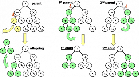
- Mutation (asexual operation) with a weak probability of the order of some percents (see figure below). It consists in randomly choosing a mutation point in the tree, and then to replace the subtree issued from this point by a new structure randomly created by the same process as in (S1).
- Crossover (sexual recombination) with a strong occurrence probability greater than 80%. During this operation, two parent individuals are selected and two crossover points are randomly chosen (one for each tree). The two subtrees rooted from these points are then exchanged to produce two offspring individuals, inheriting thus partly from each of their parents (see figure below).
- Reproduction (cloning) which simply copies the selected individual to the new population.
- Architecture-altering operations (gene duplication and deletion), each of them being applied sparingly with a weak probability less than 1%. They are motivated by the fact that the size and shape of the solution are sometimes a major part of the problem. This is especially true in our case, since the number and type of regressors' kernels will condition the tree's depth and shaping. Consequently, GP will use these operations to automatically modify the architecture of population trees, increasing their diversity with the hope that architectures well-suited to the problem will multiply and prosper under the selective pressure of the competition. These operations include duplication, creation/deletion of branches or leaves, i.e. terminal nodes and function arguments.
- (S4) Go back to (S2) following an iterative process, until a termination criterion is satisfied or a maximum number of generations N is reached. The best-so-far program produced during the run is retained as the result, and corresponds to a solution or approximate solution to the problem if the run is successful (convergence). Suboptimal results can also be favored in terms of a trade-off between performances and complexity.
As regards to the selection strategy of individuals from which the next generation will inherit, the applied techniques are similar to those used by other evolutionary methods. Therefore, several types of selection are available by:
- Uniform sampling $\rightarrow$ the selection probability obeys a uniform distribution and all individuals have the same chance to be selected regardless of their fitness.
- Roulette wheel $\rightarrow$ the selection probability is proportional to the fitness of the individuals. The best image to figure the process is a casino roulette where the better the individuals, the larger the size of the sectors. This strategy tends to favor the good elements which will be more easily selected, but can rapidly weaken the population in case of big gaps in the performance, i.e. between the best individual and the following ones.
- Fitness ranking $\rightarrow$ this a variant of the roulette wheel, aiming at increasing the diversity of the selected individuals in case of heterogenous distribution of the fitnesses (the drawback being to slow the convergence). To do that, the population is sorted by fitness at first, the individuals being ranked from 1 (the best) to $M$ (the worst). They are selected following a roulette process then, but with a probability proportional to their rank and no more to their fitness.
- Tournament $\rightarrow$ $k$ individuals are picked up at random and the best one is selected. This operation is repeated as many times as necessary to get the required number of individuals. Thus, the choice of $k$ permits to give more or less chance to the worst individuals: a high value will penalize them heavily whereas, if $k$ is low, they could be selected even so. This parameter can also be varied during the iterations to control the switch between exploration (low $k$) and exploitation stages (high $k$).
References
| [1] | A. Bucharles et al., "An overview of relevant issues for aircraft model identification", AerospaceLab, Issue 4, http://www.aerospacelab-journal.org/al4, 2012. |
| [2] | G. Hardier, C. Roos and C. Seren, "Creating sparse rational approximations for linear fractional representations using genetic programming", in Proceedings of the 3rd IFAC International Conference on Intelligent Control and Automation Science, Chengdu, China, pp. 232-237, September 2013. |
| [3] | J.R. Koza and R. Poli, "A Genetic Programming Tutorial", In Burke ed., Intoductory Tutorials in Optimization, Search and Decision Support, 2003. |
| [4] | J. Madar, J. Abonyi and F. Szeifert, "Genetic programming for the identification of nonlinear input-output models", Industrial and Engineering Chemistry Research, 44 (9), pp. 3178-3186, 2005. |
| [5] | C. Sanathanan and J. Koerner, "Transfer function synthesis as a ratio of two complex polynomials", IEEE Transactions on Automatic Control, 8 (1), pp. 56-58, 1963. |
| [6] | D.P. Searson, D.E. Lealy and M.J. Willis, "GPTIPS: an open source GP toolbox for multigene symbolic regression", International Multiconference of Engineers and Computer Scientists, Hong Kong, China, 2010. |
| [7] | C. Seren, G. Hardier and P. Ezerzere, "On-line Estimation of Longitudinal Flight Parameters", SAE AeroTech Congress and Exhibition, Toulouse, France, 2011. |

